A monitoring system that surfaces three independent exposure estimates — CHD, GDACS, ADAM — per (storm, admin unit, wind threshold) eventually has to show operators one number. The proposed rule, and the one the alert pipeline already uses, is MAX over the sources: “the highest credible estimate is the operationally relevant figure.” This chapter stress-tests that rule on the historical record.
Scope — forward-looking. We restrict to the all-three-operational era (season ≥ 2023): ADAM reports from 2023, GDACS computes per-country exposure from ~2023. Before that GDACS has systematic data gaps (see ch. 9), and mixing eras would measure coverage history rather than how MAX behaves today. In this era a missing source value is a true 0 (the source found nobody — not a coverage gap), so it is zero-filled before averaging.
It builds live from src/source_exposure (build_exposure, the harmonised workbook’s own five-case fills); no scratch-artefact dependency.
TipKey findings
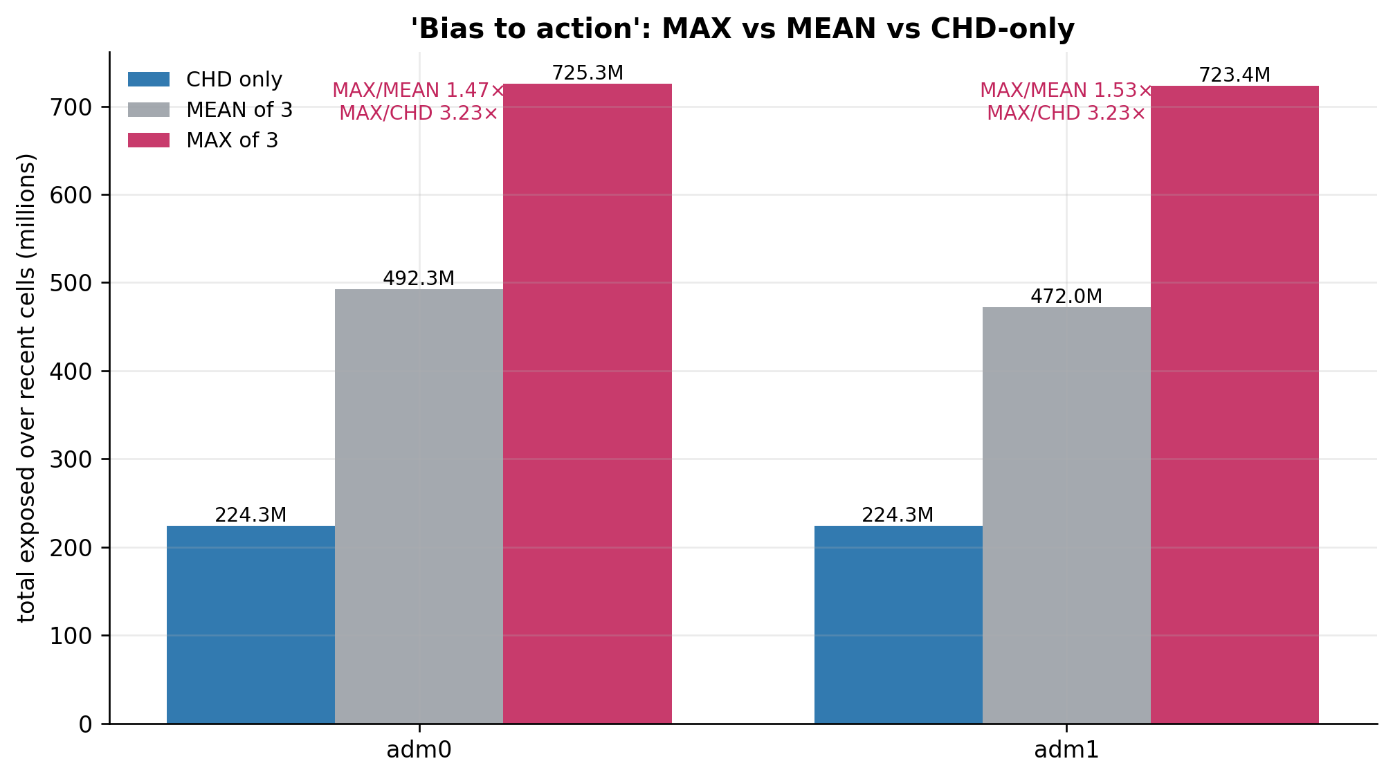
MAX roughly triples the CHD figure — total exposed under MAX-of-3 is ~3.2× the CHD-only number (and ~1.5× the mean of the three) (Figure 9.6).
The one number is almost entirely an ADAM/GDACS figure — weighted by people, ADAM supplies 68% of the country MAX and 54% subnationally, GDACS most of the rest; CHD contributes just 4–10% (Figure 9.3).
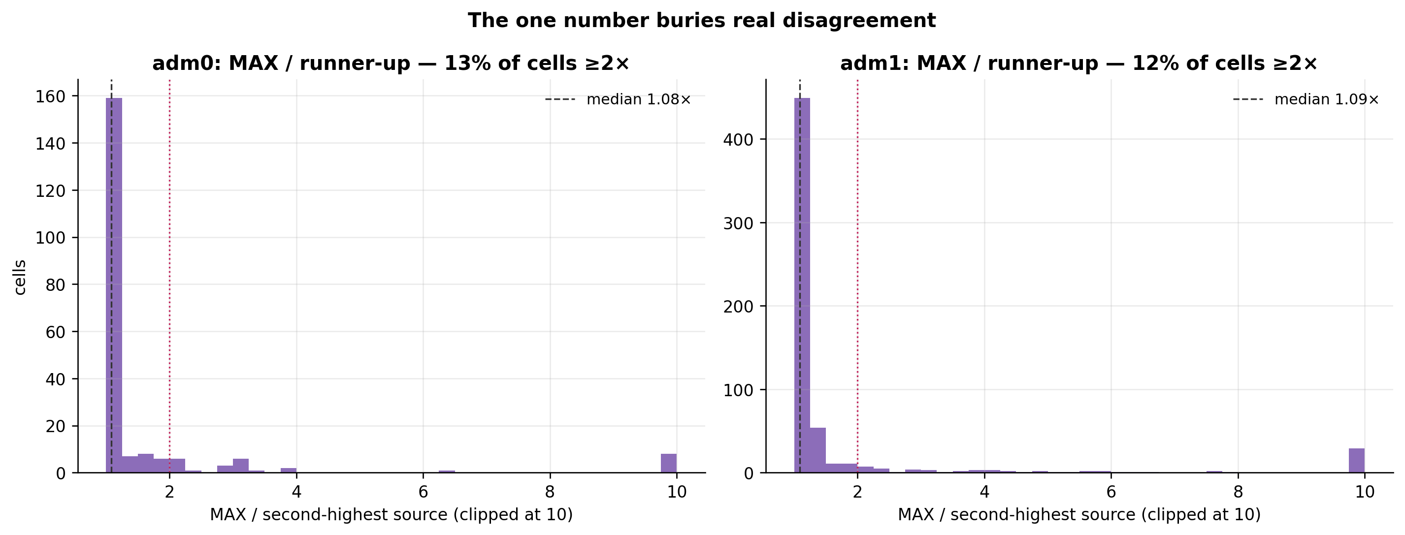
The sources usually agree — the MAX is within ~10% of the runner-up source in most cells (median ≈ 1.08×); only ~1 in 8 cells disagree ≥2×, so MAX is occasionally a large outlier (Figure 9.9).
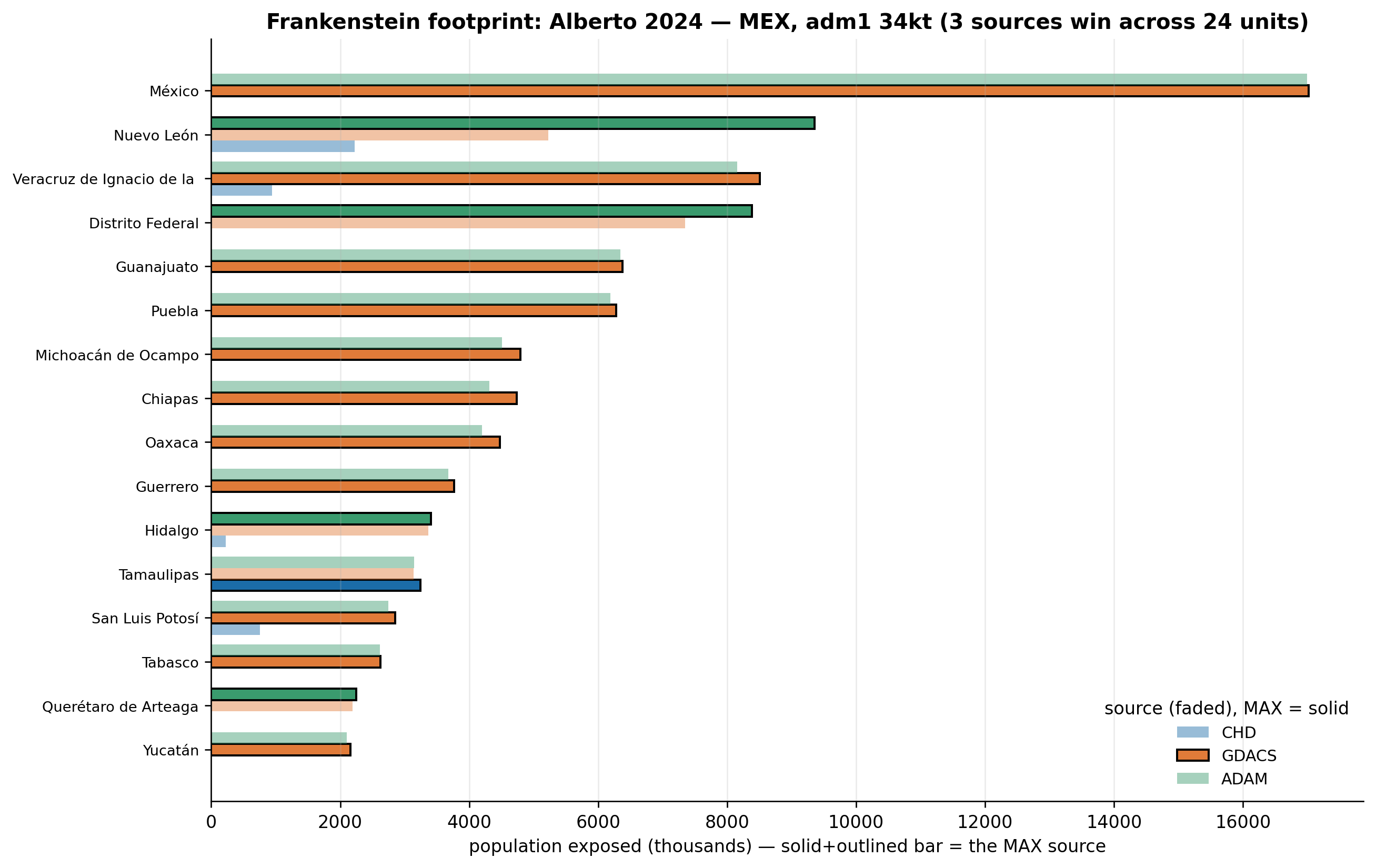
The subnational MAX surface stitches all three methodologies together — across a single storm’s admin units, CHD, GDACS and ADAM each win somewhere (Figure 9.8).
9.1 TL;DR
MAX roughly triples CHD. Over the recent era, total exposed under MAX-of-3 is ~3.2× the CHD-only figure and ~1.5× the mean of the three. “Bias to action” is not a rounding adjustment.
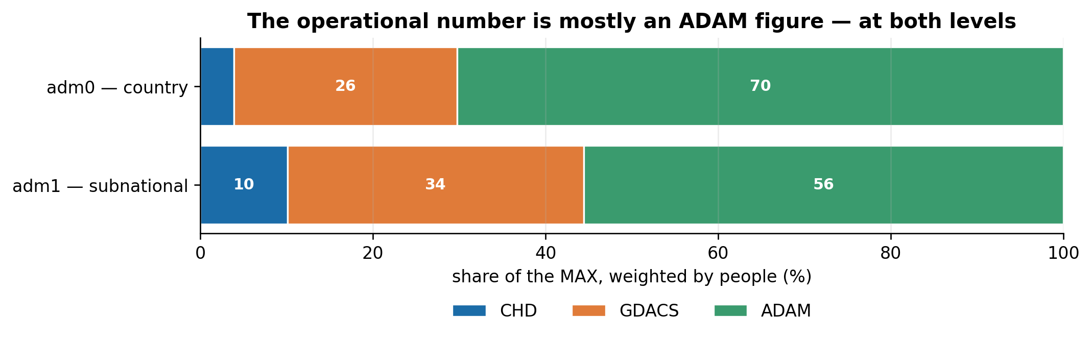
The operational number is almost entirely an ADAM/GDACS figure — at both levels. Weighted by people, ADAM supplies 68% of the adm0 MAX and 54% of the adm1 MAX, GDACS most of the rest; CHD is the smallest contributor at both (4% / 10%).
The sources usually agree closely. The MAX is within ~10% of the runner-up source in most cells (median ≈ 1.08×); only ~1 in 8 cells disagree ≥2×. So MAX is usually near-consensus, with occasional large outliers.
MAX is near-consistent across admin levels. Summing the per-adm1 MAXes exceeds the national adm0 MAX in ~33% of country-storms but almost always marginally (median ratio ≈ 1.0), with a few material exceptions where units genuinely split sources.
MAX is operationally defensible. It is not a neutral consensus number.
9.2 Method
Per cell we have up to three values. With missing = 0 (recent era):
MAX = the largest of the three (a 0 never wins, so MAX is unaffected by the zero-fill). max_source = which source achieved it.
MEAN = average of all three, denominator 3 (a source that found nobody contributes 0).
n_positive = how many of the three found anybody (1–3); it drives MAX/MEAN.
Spread/attribution use the positive sources only.
GDACS carries no 50 kt buffer, so GDACS-relevant comparisons use {34, 64} kt.
Code
import syssys.path.insert(0, "..")from dotenv import load_dotenvload_dotenv()import numpy as npimport pandas as pdimport matplotlib.pyplot as pltfrom src.source_exposure import workbook as wbfrom src.source_exposure import queries as qplt.rcParams.update({"figure.dpi": 120, "savefig.bbox": "tight", "axes.grid": True,"grid.alpha": 0.25, "axes.spines.top": False, "axes.spines.right": False,"font.size": 10, "axes.titlesize": 12, "axes.titleweight": "bold","figure.facecolor": "white"})SOURCES = ("chd", "gdacs", "adam")COL = {"chd": "chd_exposure", "gdacs": "gdacs_exposure", "adam": "adam_exposure"}LABEL = {"chd": "CHD", "gdacs": "GDACS", "adam": "ADAM"}COLOR = {"chd": "#1b6ca8", "gdacs": "#e07b39", "adam": "#3a9b6e"}VALCOLS = [COL[s] for s in SOURCES]RECENT_MIN_SEASON =2023def add_combined(df): v = df[VALCOLS] df = df.copy() df["max_val"] = v.max(axis=1) df["mean_val"] = v.mean(axis=1) df["n_sources"] = v.notna().sum(axis=1) df["n_positive"] = (v >0).sum(axis=1) df["max_source"] = v.idxmax(axis=1).map({COL[s]: s for s in SOURCES})return dfdef recent(df, zero_missing=True):"""Recent all-operational era; missing = TRUE 0 (zero-filled, so MEAN / 3).""" d = df[df["season"] >= RECENT_MIN_SEASON].copy()if zero_missing: d[VALCOLS] = d[VALCOLS].fillna(0.0) d = add_combined(d)return ddef human(n):if n isNoneor (isinstance(n, float) and np.isnan(n)):return"n/a"for div, suf in ((1e9, "B"), (1e6, "M"), (1e3, "k")):ifabs(n) >= div:returnf"{n / div:.1f}{suf}"returnf"{n:.0f}"# ── build the panels once (live from the dev DB) ─────────────────────────────eng = q.get_engine("dev")aids = q.all_nhc_storms(eng, wb.MIN_SEASON, wb.MAX_SEASON)["atcf_id"].tolist()_, gd_rep, ad_rep = q.storms_with_source_exposure(eng, aids)resolve = wb._country_resolver(eng)panel0 = wb.build_exposure(eng, 0, aids, gd_rep, ad_rep, resolve)panel1 = wb.build_exposure(eng, 1, aids, gd_rep, ad_rep, resolve)R0 = recent(panel0) # adm0, recent era, missing=0R1 = recent(panel1) # adm1, recent era, missing=0KT = R0.wind_speed_kt.isin([34, 64])n_storms = recent(panel0)["atcf_id"].nunique()
The recent era covers 62 storms (seasons 2023–2026) with all three systems live.
9.3 1. Summing subnational MAXes can exceed the national MAX — usually marginally
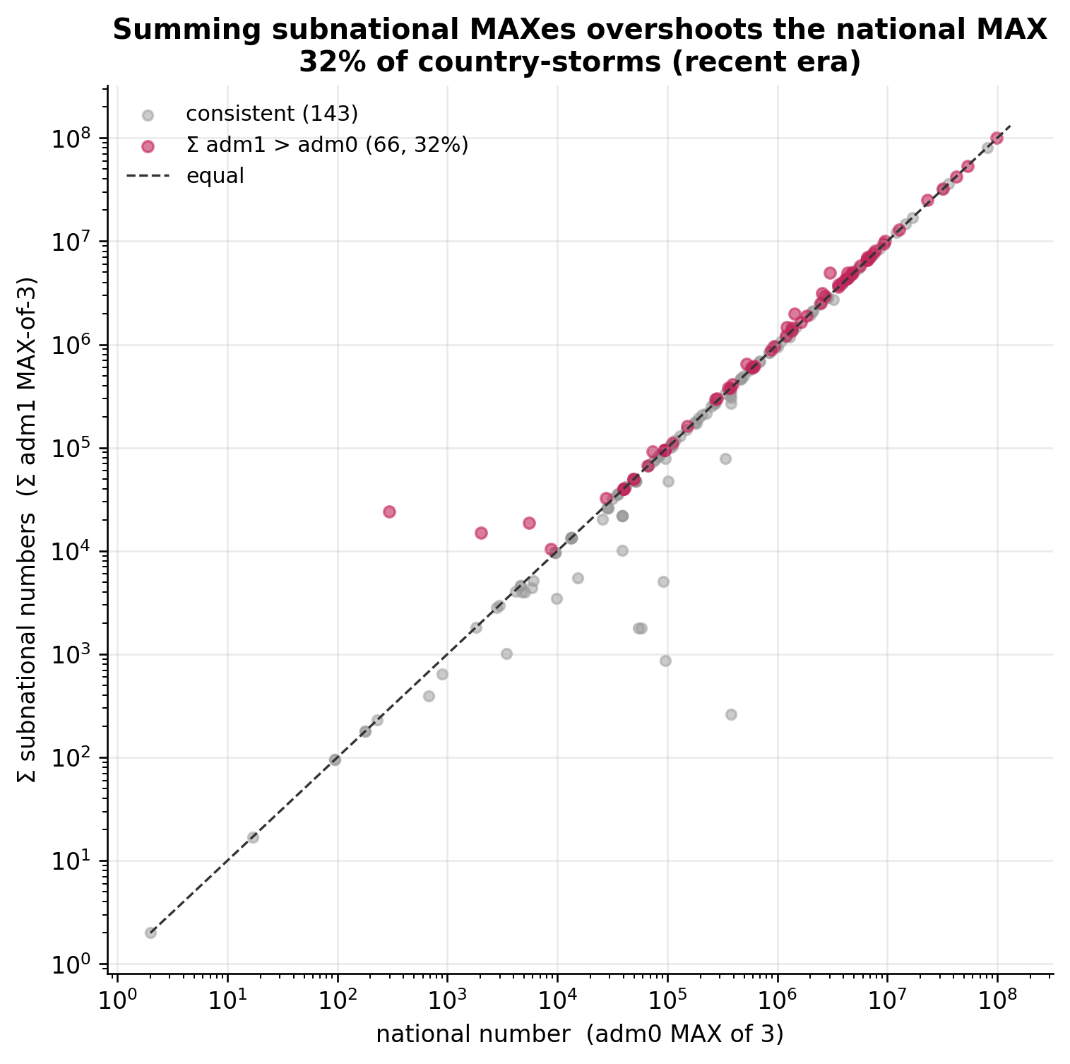
A screen shows, per country, an adm0 number (MAX of the three) and a set of adm1 numbers (each the MAX of the three). Sum the adm1 numbers and they can exceed the adm0 number — because each subnational unit may pick a different source as its max (sum-of-maxes ≥ max-of-sums). This is structural, not a bug, and in practice small: CHD now reconciles exactly across levels (a country’s adm0 value equals the sum of its adm1 units), so the only thing driving an overshoot is per-unit source-switching — a modest effect, with a few real exceptions.
The scatter also has points below the diagonal — country-storms where the subnational sum falls short of the national MAX. These arise because GDACS and (to a lesser extent) ADAM do not fully reconstitute their national totals subnationally: their adm1 footprints are sparser than their adm0 figure, so when one of them sets the national MAX, the per-unit MAXes can’t recover it. (CHD, which conserves exactly, never causes this.) It is the external-source mirror of the same admin-level reconciliation issue — modest, but worth knowing the screen won’t perfectly tie out in either direction.
Figure 9.1: Per (storm, country, threshold): the national MAX vs the sum of the per-adm1 MAXes (recent era). Points above the diagonal are country-storms where the subnational total overshoots the national number — about a third of them, and nearly all only marginally (the cloud hugs the diagonal).
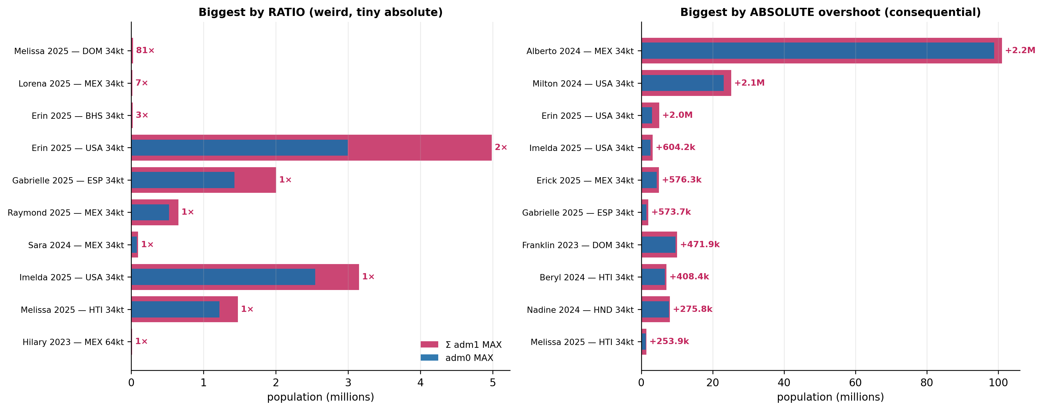
Figure 9.2: Two faces of the overshoot. Left: largest by ratio — extreme but tiny-absolute (the national number is ~0). Right: largest by absolute overshoot — the operationally consequential few (Cristina/GTM adds ~6M people subnationally vs nationally; Alberto/MEX ~2M).
The median ratio is 1.0 and the 90th percentile only ~1.06× — for almost all country-storms the subnational sum matches the national MAX. The exceptions are a handful where admin units genuinely split across sources: Cristina 2026 (Guatemala) adds ~6M people subnationally, Alberto 2024 (Mexico) ~2M. So a user summing the subnational screen will usually land on the national figure, but should expect it to run a little high — and occasionally much higher.
9.4 2. Who drives the MAX — it’s mostly an ADAM number
Weighted by people — the population that actually lands in the operational number — the MAX is almost entirely an ADAM/GDACS figure at both the country (adm0) and subnational (adm1) level: ADAM supplies 68% of the exposed people at adm0 and 54% at adm1, GDACS most of the rest (28% / 37%), and CHD the smallest contributor at both (4% and 10%). The GDACS-family drives the number whether you look at the country or the subnational level. (Counting cells instead of people shifts the shares a little, but that is a coverage-breadth diagnostic, not the number — see the foldable note below.)
Code
def shares(d): bc = d.max_source.value_counts(normalize=True) bp = d.groupby("max_source").max_val.sum(); bp = bp / bp.sum()return bc, bpd0 = R0[KT & (R0.max_val >0)]d1 = R1[R1.wind_speed_kt.isin([34, 64]) & (R1.max_val >0)]def plot_shares(groups, xlabel, title): fig, ax = plt.subplots(figsize=(9, 3.1)) y = np.arange(len(groups))[::-1]; left = np.zeros(len(groups))for s in SOURCES: vals = np.array([g_[1].get(s, 0) *100for g_ in groups]) ax.barh(y, vals, left=left, color=COLOR[s], label=LABEL[s], edgecolor="white")for yi, v, l inzip(y, vals, left):if v >5: ax.text(l + v /2, yi, f"{v:.0f}", ha="center", va="center", color="white", fontsize=9, fontweight="bold") left += vals ax.set_yticks(y); ax.set_yticklabels([g_[0] for g_ in groups]) ax.set_xlim(0, 100); ax.set_xlabel(xlabel); ax.set_title(title) ax.legend(ncol=3, frameon=False, loc="upper center", bbox_to_anchor=(0.5, -0.28)) ax.grid(axis="y", visible=False); fig.tight_layout() plt.show()plot_shares([("adm0 — country", shares(d0)[1]), ("adm1 — subnational", shares(d1)[1])],"share of the MAX, weighted by people (%)","The operational number is mostly an ADAM figure — at both levels")
Figure 9.3: Share of the MAX weighted by PEOPLE — the exposed population that lands in the operational number — at country (adm0) and subnational (adm1) level. ADAM supplies the most people at both levels (68% / 54%), GDACS most of the rest; CHD the least (4% / 10%).
Code
nmcol ="country_name"if"country_name"in d0 else"iso3"cc = d0.groupby([nmcol, "max_source"]).max_val.sum().unstack(fill_value=0)cc = cc.loc[cc.sum(axis=1).sort_values(ascending=False).head(14).index]frac = cc.div(cc.sum(axis=1), axis=0)fig, ax = plt.subplots(figsize=(9.5, 6)); yy = np.arange(len(frac))[::-1]left = np.zeros(len(frac))for s in SOURCES: vals = frac.get(s, pd.Series(0, index=frac.index)).values *100 ax.barh(yy, vals, left=left, color=COLOR[s], label=LABEL[s], edgecolor="white") left += valsax.set_yticks(yy)ax.set_yticklabels([f"{i}"for i in frac.index], fontsize=8.6)ax.set_xlim(0, 100); ax.set_xlabel("share of country MAX people (%)")ax.set_title("Provenance of the country MAX is country-specific")ax.legend(ncol=3, frameon=False, loc="upper center", bbox_to_anchor=(0.5, -0.1))ax.grid(axis="y", visible=False)fig.tight_layout()plt.show()
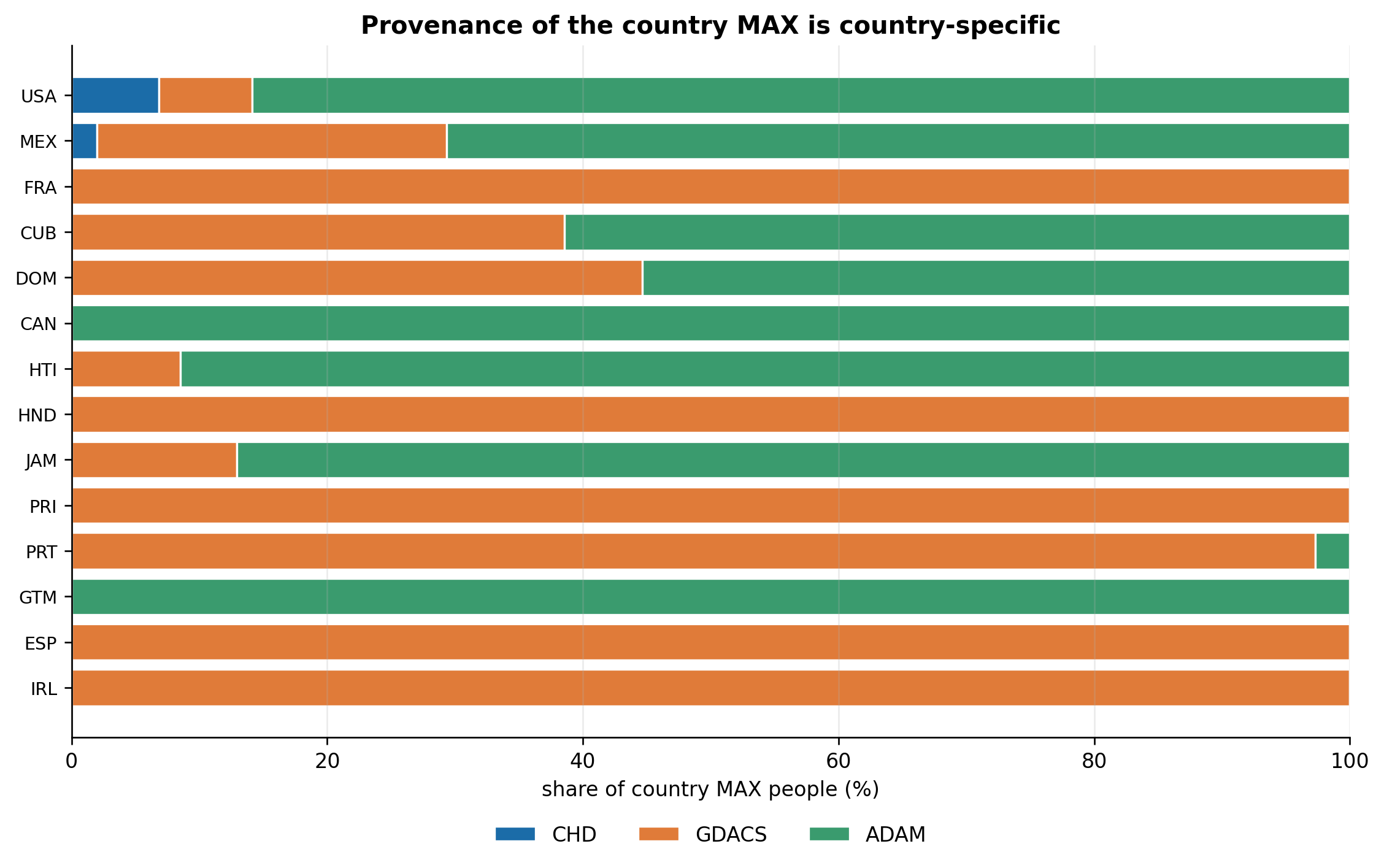
Figure 9.4: Which source supplies the country (adm0) MAX population, by country (top 14 by exposed people). It varies a lot — some countries are ADAM-driven, others CHD or GDACS — so the operational number’s provenance is country-specific.
NoteDiagnostic: who wins the most cells (coverage breadth, not the number)
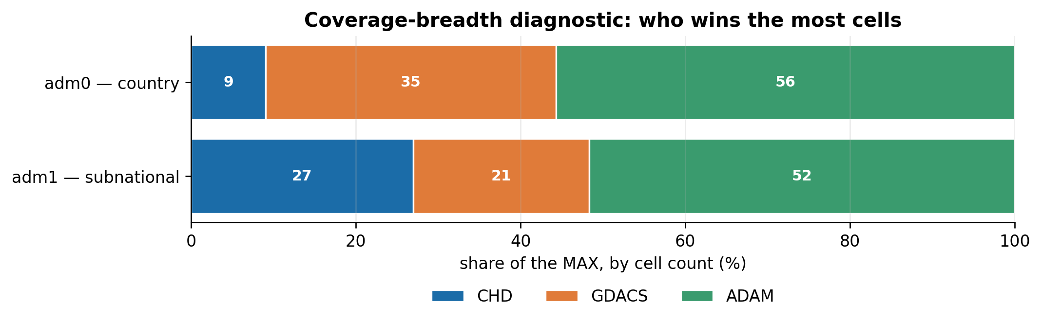
Counting how often each source wins a cell — regardless of how many people are in it — measures coverage breadth, not the operational number. ADAM leads on cells at both levels (55% adm0, 51% adm1). CHD’s cell share (9% adm0, 26% adm1) runs well above its people share (4% / 10%): it reaches many small admin units the others don’t, but those cells carry few people, so they barely lift the population-weighted number. That gap between the cell view and the people view flags CHD’s broad-but-thin subnational footprint.
Code
plot_shares([("adm0 — country", shares(d0)[0]), ("adm1 — subnational", shares(d1)[0])],"share of the MAX, by cell count (%)","Coverage-breadth diagnostic: who wins the most cells")
Figure 9.5: Diagnostic — share of the MAX by CELL COUNT (who wins most often, ignoring population). ADAM leads at both levels (55% adm0, 51% adm1); CHD’s cell share (9% / 26%) exceeds its people share, reflecting many small units. Compare with the by-people view above.
9.5 3. MAX vs MEAN vs CHD-alone — the “bias to action” cost
Code
P = {"adm0": d0, "adm1": d1}fig, ax = plt.subplots(figsize=(8.5, 4.8)); x = np.arange(2); w =0.26for i, (lab, col, color) inenumerate( [("CHD only", "chd_exposure", "#1b6ca8"), ("MEAN of 3", "mean_val", "#9aa0a6"), ("MAX of 3", "max_val", "#c2255c")]): tot = [P["adm0"][col].sum() /1e6, P["adm1"][col].sum() /1e6] b = ax.bar(x + (i -1) * w, tot, w, label=lab, color=color, alpha=0.9)for rect, v inzip(b, tot): ax.text(rect.get_x() + rect.get_width() /2, v, human(v *1e6), ha="center", va="bottom", fontsize=8.5)for k, xi in (("adm0", 0), ("adm1", 1)): d = P[k] ax.text(xi, ax.get_ylim()[1] *0.9,f"MAX/MEAN {d.max_val.sum()/d.mean_val.sum():.2f}×\n"f"MAX/CHD {d.max_val.sum()/d.chd_exposure.sum():.2f}×", ha="center", fontsize=8.5, color="#c2255c")ax.set_xticks(x); ax.set_xticklabels(["adm0", "adm1"])ax.set_ylabel("total exposed over recent cells (millions)")ax.set_title("'Bias to action': MAX vs MEAN vs CHD-only")ax.legend(frameon=False, fontsize=9)fig.tight_layout()plt.show()
Figure 9.6: Total exposed over recent-era cells under CHD-only, MEAN-of-3, and MAX-of-3. Adopting MAX roughly triples the CHD figure (3.24× adm0, 3.27× adm1) and is ~1.5× the mean. CHD is identical at adm0 and adm1 (232M) — it reconciles across levels.
Code
fig, axes = plt.subplots(1, 2, figsize=(12, 4.6))for ax, (k, d) inzip(axes, P.items()): d = d[d.mean_val >0].copy(); d["infl"] = d.max_val / d.mean_valfor npos, color in ((1, "#c2255c"), (2, "#e07b39"), (3, "#3a9b6e")): sub = d[d.n_positive == npos]iflen(sub): ax.hist(sub.infl, bins=np.linspace(1, 3.05, 30), alpha=0.65, color=color, label=f"{npos} of 3 found people (n={len(sub)})") ax.set_title(f"{k}: MAX / MEAN per cell (median {d.infl.median():.2f}×)") ax.set_xlabel("MAX / MEAN (= 3 when only one source finds anybody)") ax.legend(frameon=False, fontsize=8.5, title="sources finding > 0")axes[0].set_ylabel("cells")fig.suptitle("MAX-over-MEAN is driven by how many sources found anybody", fontsize=12, fontweight="bold")fig.tight_layout()plt.show()
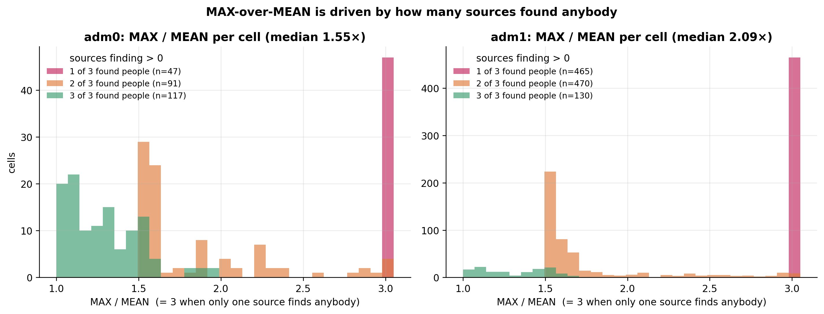
Figure 9.7: Per-cell MAX/MEAN, split by how many of the three sources found anybody. With missing=0 the mean divides by 3, so when only ONE source finds people MAX = exactly 3× the mean (the spike at 3.0); when all three agree it sits near 1×. Median MAX/MEAN ≈ 1.55× (adm0), 1.85× (adm1).
Over the recent era: adm0 totals are CHD 232M / MEAN 511M / MAX 750M (MAX/MEAN 1.47, MAX/CHD 3.24); adm1 CHD 232M / MEAN 495M / MAX 757M (1.53, 3.27). CHD’s total is the same at both levels — it reconciles across admin units — while the MAX more than triples it. The subnational median MAX/MEAN of 1.85× reflects how many adm1 cells are carried by just one or two of the three sources.
9.6 4. The “Frankenstein footprint”
Within a single storm-country the per-unit MAX can come from different sources, so the operational subnational surface is three methodologies stitched together.
Code
d = R1[(R1.wind_speed_kt ==34) & (R1.max_val >0) & (R1.n_positive >=2)].copy()gg = d.groupby(["atcf_id", "iso3"]).agg( units=("max_val", "size"), nwin=("max_source", "nunique"), ppl=("max_val", "sum"), name=("storm_name", "first")).reset_index()pick = gg[(gg.units >=6) & (gg.nwin >=2)].sort_values( ["nwin", "ppl"], ascending=False).iloc[0]sub = d[(d.atcf_id == pick.atcf_id) & (d.iso3 == pick.iso3)]sub = sub.sort_values("max_val", ascending=False).head(16).iloc[::-1]fig, ax = plt.subplots(figsize=(11, 7)); y = np.arange(len(sub)); h =0.26for i, s inenumerate(SOURCES): vals = sub[COL[s]].fillna(0).to_numpy() /1e3 bars = ax.barh(y + (i -1) * h, vals, h, color=COLOR[s], alpha=0.45, label=LABEL[s])for (_, r), rect inzip(sub.iterrows(), bars):if r.max_source == s: rect.set_alpha(1.0); rect.set_edgecolor("black"); rect.set_linewidth(1.2)ax.set_yticks(y); ax.set_yticklabels([str(n)[:26] for n in sub.admin_name], fontsize=8.2)ax.set_xlabel("population exposed (thousands) — solid+outlined bar = the MAX source")ax.set_title(f"Frankenstein footprint: {pick['name'].title()} "f"{pick.atcf_id[-4:]} — {pick.iso3}, adm1 34kt "f"({int(pick.nwin)} sources win across {int(pick.units)} units)")ax.legend(frameon=False, fontsize=9, title="source (faded), MAX = solid")ax.grid(axis="y", visible=False)fig.tight_layout()plt.show()
Figure 9.8: Alberto 2024 over Mexico, adm1 34kt: each state’s three source values; the solid+outlined bar is the operational MAX. Across 24 states all three sources win somewhere — the displayed surface is a patchwork.
9.7 5. What the one number hides
Code
def max_over_second(d): out = []for row in d[VALCOLS].to_numpy(float): pos = np.sort(row[~np.isnan(row)])[::-1]; pos = pos[pos >0]iflen(pos) >=2and pos[1] >0: out.append(pos[0] / pos[1])return np.array(out)fig, axes = plt.subplots(1, 2, figsize=(12, 4.6))for ax, (k, d) inzip(axes, P.items()): r = max_over_second(d) ax.hist(np.clip(r, 1, 10), bins=np.linspace(1, 10, 37), color="#7048a8", alpha=0.8) ax.axvline(np.median(r), color="#333", ls="--", lw=1, label=f"median {np.median(r):.2f}×") ax.axvline(2, color="#c2255c", ls=":", lw=1) ax.set_title(f"{k}: MAX / runner-up — {(r >=2).mean()*100:.0f}% of cells ≥2×") ax.set_xlabel("MAX / second-highest source (clipped at 10)") ax.legend(frameon=False, fontsize=9)axes[0].set_ylabel("cells")fig.suptitle("The one number buries real disagreement", fontsize=12, fontweight="bold")fig.tight_layout()plt.show()
Figure 9.9: MAX divided by the second-highest source, on cells where ≥2 sources found people. The chosen number is ≥2× the runner-up in ~13% (adm0) / ~12% (adm1) of cells (median ≈ 1.08×) — most of the time the sources are close, but a minority disagree sharply.
9.8 Implications
MAX is a reasonable operational default — for alerting you want the highest credible figure, and MAX guarantees no source’s warning is missed. But it should be read for what it is, not as a neutral consensus:
It is roughly 3× CHD and 1.5× the mean — adopting it shifts the headline exposure number materially upward, era-wide.
It is almost entirely an ADAM/GDACS figure at both levels (ADAM = 68% of adm0 people, 54% at adm1; CHD just 4–10%), so the operational number inherits the GDACS-family’s wind-polygon methodology, not CHD’s wind-radii one.
It is near-consistent across admin levels — each source now reconciles adm0 = Σadm1, so the subnational screen exceeds the national figure only marginally (a third of country-storms, almost always by a few percent).
It usually tracks the consensus, but occasionally not — the MAX is within ~10% of the runner-up in most cells, yet ≥2× the runner-up in ~1 in 8, so MAX alone gives no signal of confidence.
A monitoring system can keep MAX as the action number while (a) showing the three sources and the spread alongside it so operators see the uncertainty, and (b) labelling provenance (which source drove the number) given how overwhelmingly it is ADAM/GDACS.