12Old exposure comparison (OCHA vs GDACS, superseded)
Two population-exposure datasets are available to us for tropical cyclones at the national level: the OCHA in-house product (adm0_ibtracs_exp_all.parquet) and the GDACS historical national exposure table. Both attach a population figure to a (storm, country, wind-threshold) tuple, but they are produced by different pipelines and do not agree on which tuples exist or on what those populations are.
This chapter compares the two methods. The goal is not to pick a winner but to characterise where they overlap, where they diverge, and by how much. We restrict to 2022 onward, because the GDACS historical CSV does not have usable values before 2022 (see the RR allocation appendix for why).
The different encoding of “no exposure” is important. A missing OCHA row does not mean zero population was exposed; it means OCHA’s methodology did not produce a value for that storm-country-threshold combination. Treating missing rows as zero would fabricate agreement or disagreement depending on which side has more coverage.
12.2 Setup
Code
import matplotlib.pyplot as pltimport matplotlib.ticker as mtickerimport numpy as npimport ocha_stratus as stratusimport pandas as pdfrom dotenv import load_dotenvload_dotenv()plt.rcParams.update({"figure.dpi": 110, "axes.grid": True, "grid.alpha": 0.3})ocha = stratus.load_parquet_from_blob("ds-storm-impact-harmonisation/processed/adm0_ibtracs_exp_all.parquet")gdacs = stratus.load_csv_from_blob("ds-cyclone-exposure/gdacs_historical_national_exposure.csv")
Code
ocha["year"] = ocha["sid"].str[:4].astype(int)ocha22 = ocha[ocha["year"] >=2022].copy()gdacs22 = gdacs[gdacs["season"] >=2022].copy()# GDACS uses -1 as a sentinel for missing; treat as null.for col in ["pop_34kt", "pop_64kt"]: gdacs22.loc[gdacs22[col] <0, col] = np.nan# OCHA wide: one row per (sid, iso3) with 34 and 64 kt columns.# 50 kt is dropped because GDACS has no equivalent.ocha_wide = ( ocha22[ocha22["speed"].isin([34, 64])] .pivot_table( index=["sid", "ADM0_A3"], columns="speed", values="pop_exposed", ) .reset_index() .rename(columns={"ADM0_A3": "iso3", 34: "ocha_34", 64: "ocha_64"}))g_wide = gdacs22[["sid", "iso3", "season", "name", "pop_34kt", "pop_64kt"]].rename( columns={"pop_34kt": "gdacs_34", "pop_64kt": "gdacs_64"})pairs = ocha_wide.merge(g_wide, on=["sid", "iso3"], how="outer", indicator=True)pairs["season"] = pairs["season"].fillna(pairs["sid"].str[:4].astype(float))pairs["year"] = pairs["season"].astype(int)def sid_to_basin(sid) ->str:"""Infer genesis basin from IBTrACS SID. SID encodes genesis hemisphere at position 7 and genesis longitude (0–360) at positions 10–13. Rough basin bins below suffice for the NA vs EP comparison we care about; other basins are grouped but not sub-divided precisely. """ifnotisinstance(sid, str) orlen(sid) <13:return"unknown" hemi = sid[7]try: lon =int(sid[10:13])exceptValueError:return"unknown"if hemi =="N":if lon >=261or lon <20:return"NA"if180<= lon <261:return"EP"if100<= lon <180:return"WP"if30<= lon <100:return"NI"return"other"if20<= lon <135:return"SI"if135<= lon <210:return"SP"return"other"pairs["basin"] = pairs["sid"].map(sid_to_basin)
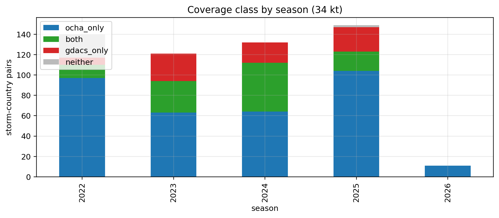
Read this as: of 553 storm-country pairs active in 2022+ in at least one dataset, only ~20% have a value on both sides at 34 kt, and far fewer at 64 kt. OCHA-only dominates at 34 kt, meaning the GDACS CSV is missing many storm-country pairs that OCHA records.
12.3.1 Coverage by season
Code
yr34 = ( pairs.groupby(["year", "cls_34"]).size().unstack(fill_value=0) .reindex(columns=CLASS_ORDER, fill_value=0))ax = yr34.plot.bar( stacked=True, color=[CLASS_COLORS[c] for c in yr34.columns], figsize=(9, 4),)ax.set_ylabel("storm-country pairs")ax.set_xlabel("season")ax.set_title("Coverage class by season (34 kt)")ax.legend(title=None, loc="upper left")plt.tight_layout()plt.show()
Storm-country pair coverage at 34 kt, by storm season.
12.3.2 Coverage by country (top 20 by total pair count)
Code
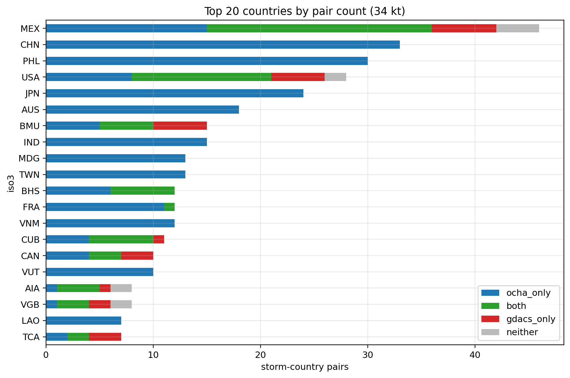
iso34 = ( pairs.groupby(["iso3", "cls_34"]).size().unstack(fill_value=0) .reindex(columns=CLASS_ORDER, fill_value=0))iso34["total"] = iso34.sum(axis=1)iso34 = iso34.sort_values("total", ascending=False).head(20).drop(columns="total")ax = iso34.plot.barh( stacked=True, color=[CLASS_COLORS[c] for c in iso34.columns], figsize=(9, 6),)ax.invert_yaxis()ax.set_xlabel("storm-country pairs")ax.set_title("Top 20 countries by pair count (34 kt)")ax.legend(title=None, loc="lower right")plt.tight_layout()plt.show()
Top 20 countries by total storm-country pairs, 2022+.
The shape of the problem is visible here: Philippines, China, Japan, Vietnam, the US Gulf-and-Caribbean belt dominate the counts. OCHA-only (blue) bars are large for West-Pacific countries. GDACS-only (red) bars, where present, tend to concentrate on Atlantic-basin coasts.
12.4 Investigating the GDACS-only pairs
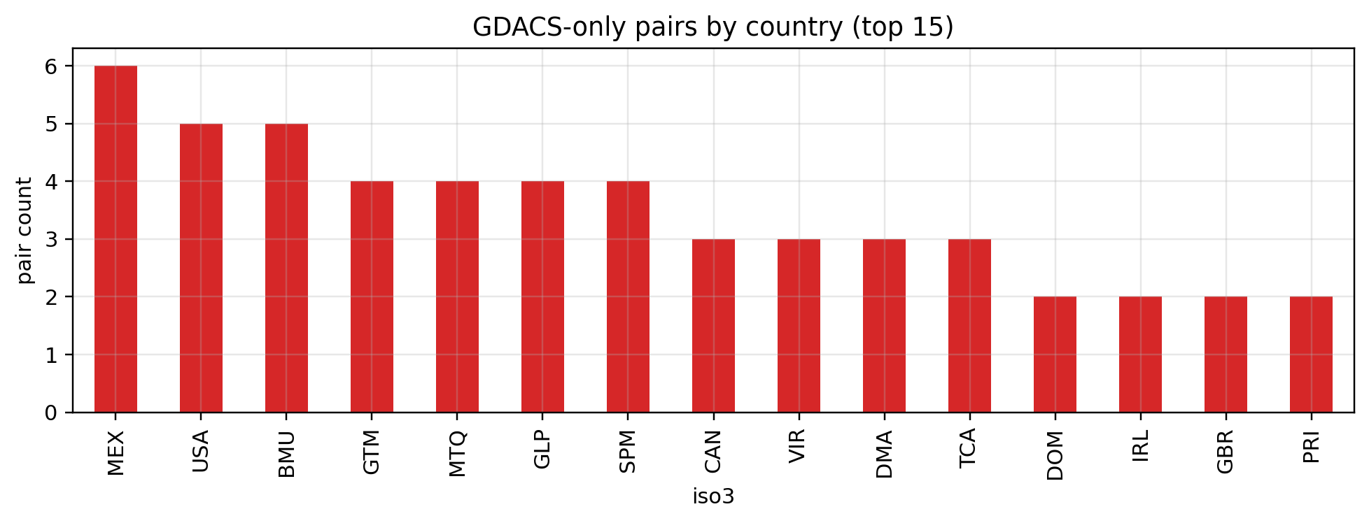
These are storm-country pairs where GDACS reports a population exposure but OCHA has no row for that (sid, iso3, speed) combination. We cannot assume OCHA measured zero; more likely, OCHA’s methodology excluded the combination. Candidates for exclusion: subtropical storms, post-tropical / extratropical stages, and cyclones that did not make formal landfall.
top = g_only_34["iso3"].value_counts().head(15)ax = top.plot.bar(color=CLASS_COLORS["gdacs_only"], figsize=(9, 3.5))ax.set_ylabel("pair count")ax.set_title("GDACS-only pairs by country (top 15)")plt.tight_layout()plt.show()
Countries most often appearing as GDACS-only at 34 kt.
A split emerges, but the interpretation got refined after the followup work documented in the appendix. Most GDACS-only pairs (about 66 of 77 in NA + EP) come from storms that are not in OCHA’s event roster at all. GDACS tracked 129 unique NA + EP storms in 2022 onward; OCHA tracked 76. The 66 missing-from- OCHA storms are disproportionately subtropical systems, open-ocean Atlantic storms, and extratropical transitions (MARTIN 2022, DANIELLE 2022, PHILIPPE 2023 post-tropical reach, ERIN 2025 post-tropical reach). For the 63 storms both datasets track, per-iso3 divergence is smaller and reflects polygon shape and phase-filter differences rather than whole-storm exclusion.
12.5 Investigating the OCHA-only pairs
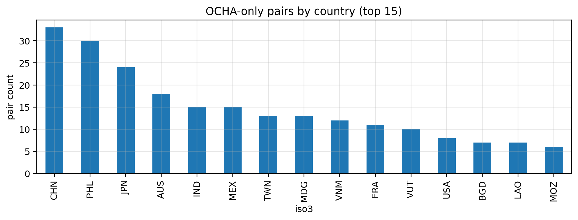
These are pairs where OCHA has exposure values but GDACS’s CSV has no usable value. Followup work (see the appendix) broke this into three sub-causes with different fixes.
top = o_only_34["iso3"].value_counts().head(15)ax = top.plot.bar(color=CLASS_COLORS["ocha_only"], figsize=(9, 3.5))ax.set_ylabel("pair count")ax.set_title("OCHA-only pairs by country (top 15)")plt.tight_layout()plt.show()
Countries most often appearing as OCHA-only at 34 kt.
The OCHA-only pattern is the opposite of GDACS-only: dominated by West Pacific and Bay of Bengal countries (PHL, CHN, VNM, JPN, BGD, KOR). These are unambiguously major tropical cyclone impacts with very large population exposure. The explanation is a deliberate filter in Hannah’s pipeline: the CSV builder hard-codes source = "NOAA", which captures only North Atlantic and Eastern Pacific events. Every WP, Indian Ocean, and Southern Hemisphere pair in OCHA is out of scope by construction, not missing by error. (See the appendix for the exact pipeline line.)
12.6 Agreement on matched pairs
Restricting to pairs where both datasets report a value, how well do the numbers agree?
12.6.1 34 kt scatter with marginal rugs for unmatched pairs
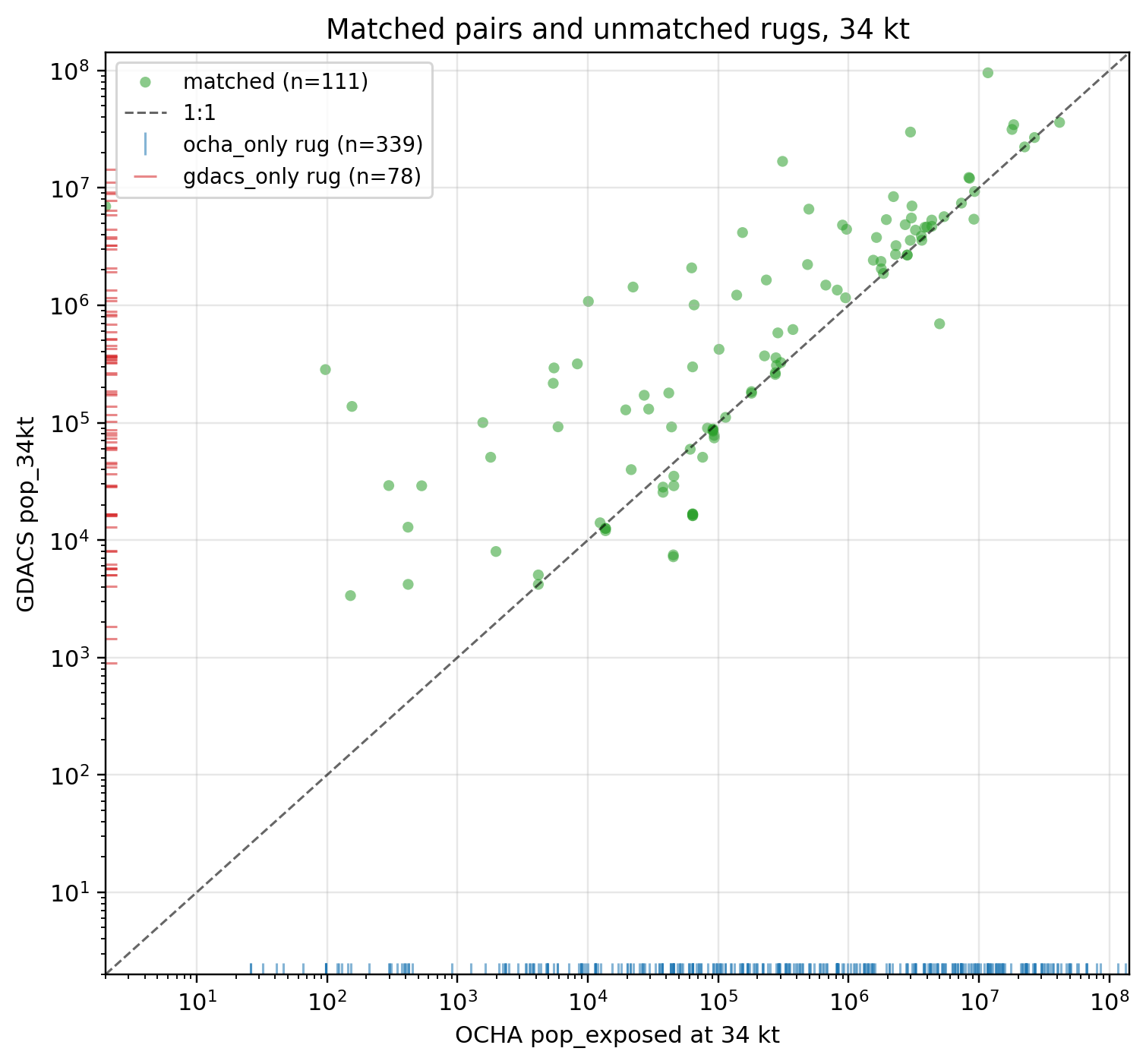
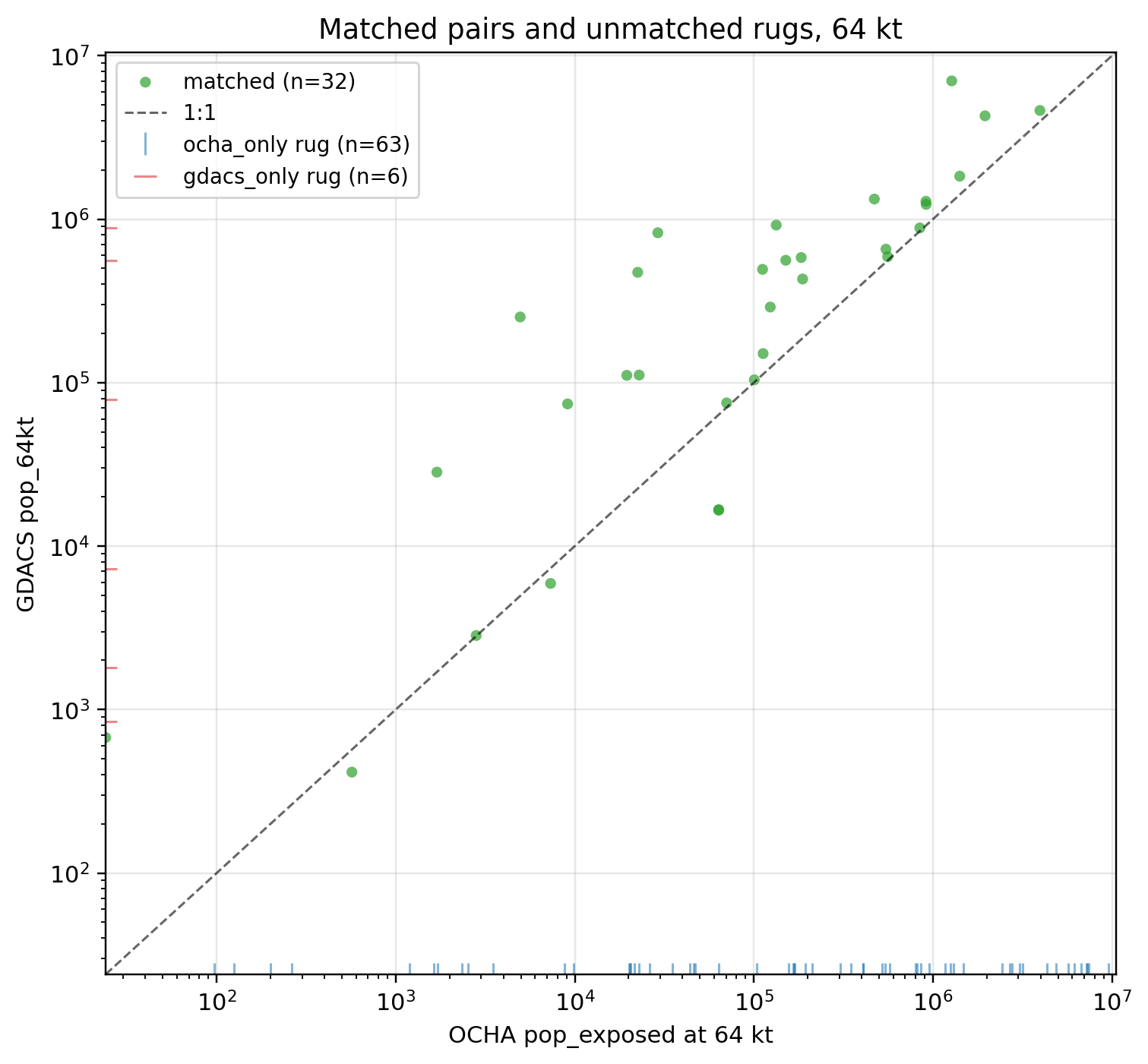
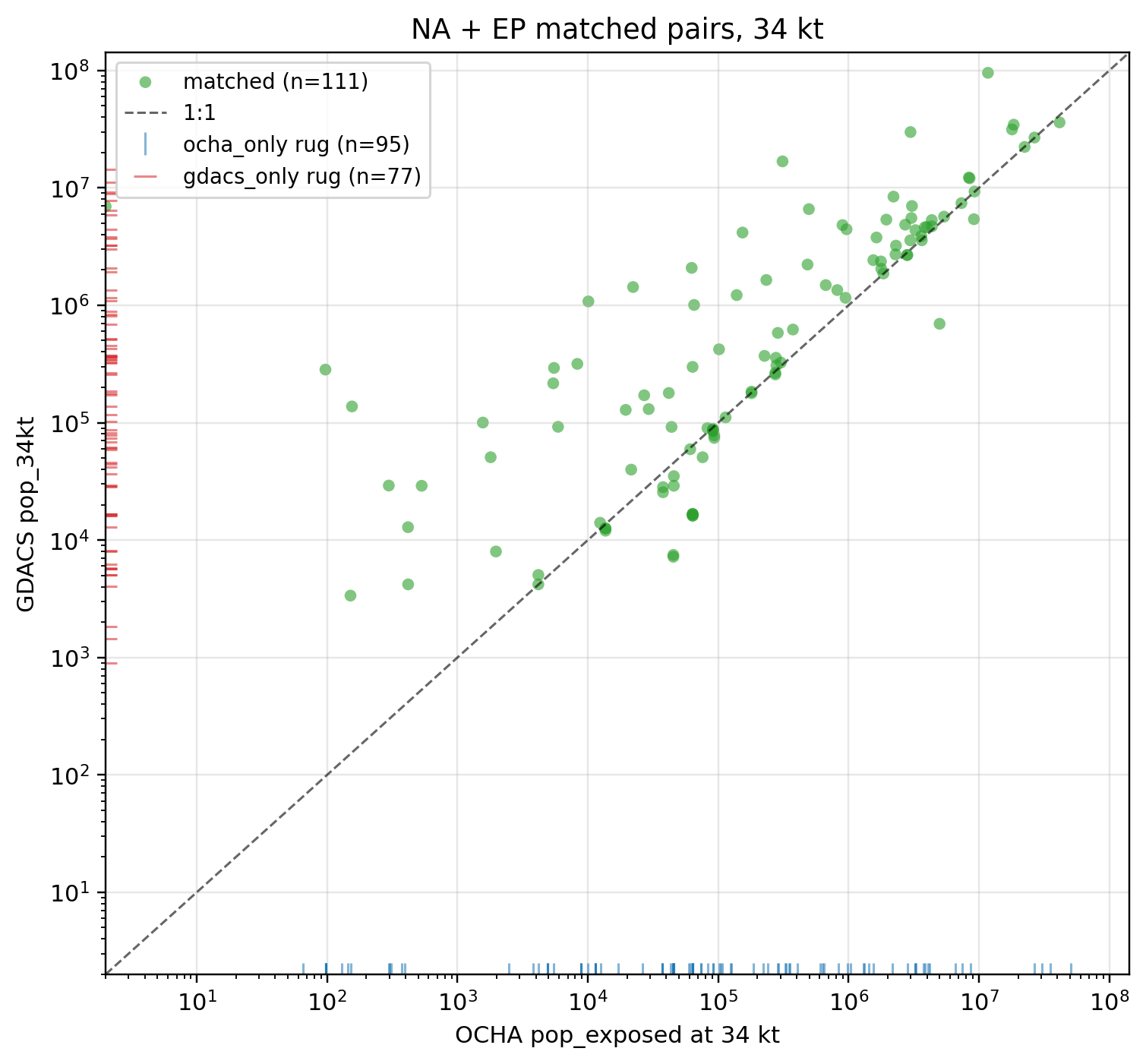
Points are matched pairs (N = 111). Marginal ticks show the pop_exposed values for pairs that only exist on one side. A point sitting far from the diagonal, or a rug extending into a region with no matched points, is where the two datasets disagree.
12.7 Restricted to North Atlantic and Eastern Pacific
Outside NA and EP, differences between OCHA and GDACS are hard to interpret: the GDACS historical CSV is effectively basin-filtered to the Atlantic and Eastern Pacific. There are no matched pairs in the Western Pacific, Indian Ocean, or Southern Hemisphere in the CSV at all, so the “OCHA-only” bars for those regions in the earlier plots do not represent methodology failures; they are simply out of CSV scope.
Because the GDACS CSV already contains only NA and EP pairs in practice, the matched-pair agreement statistics below are identical to the global ones shown earlier. The value of restricting is different: it lets us look at coverage within NA and EP, where GDACS has scope, and ask why some pairs in those basins are still OCHA-only or GDACS-only. That is a methodology question.
Note how the ocha_only category shrinks dramatically when restricted to NA + EP: most of the “missing-from-GDACS” complaint from the global view was West Pacific and Indian Ocean storms that the GDACS CSV simply did not record.
12.7.2 Coverage by season
Code
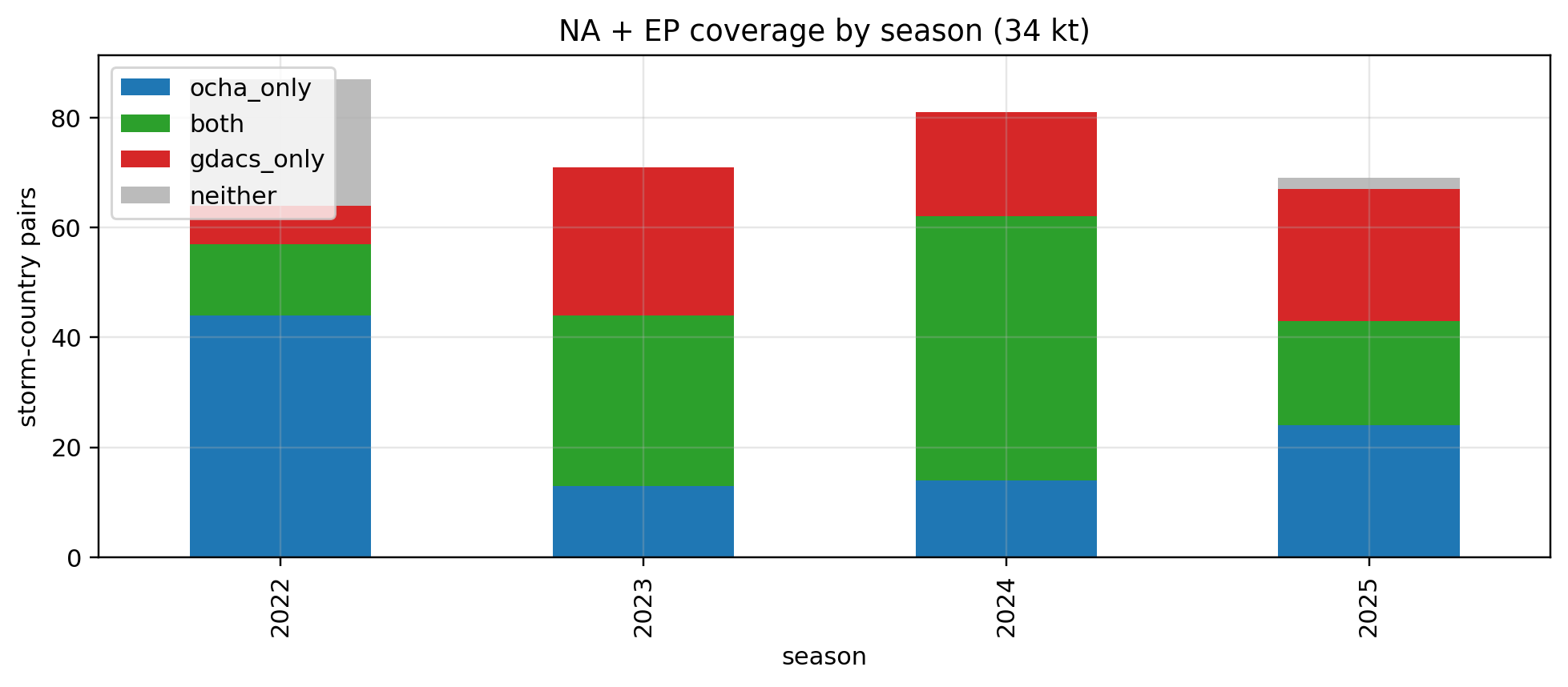
yr_ae = ( pairs_ae.groupby(["year", "cls_34"]).size().unstack(fill_value=0) .reindex(columns=CLASS_ORDER, fill_value=0))ax = yr_ae.plot.bar( stacked=True, color=[CLASS_COLORS[c] for c in yr_ae.columns], figsize=(9, 4),)ax.set_ylabel("storm-country pairs")ax.set_xlabel("season")ax.set_title("NA + EP coverage by season (34 kt)")ax.legend(title=None, loc="upper left")plt.tight_layout()plt.show()
NA + EP storm-country pair coverage at 34 kt, by season.
stats_ae = pd.DataFrame( {"34 kt (NA + EP)": agreement_stats(m34_ae, "ocha_34", "gdacs_34"),"64 kt (NA + EP)": agreement_stats(m64_ae, "ocha_64", "gdacs_64"), }).Tstats_ae
n
median(GDACS / OCHA)
corr(log OCHA, log GDACS)
pct within 2x
pct within 10x
34 kt (NA + EP)
111.0
1.333
0.724
55.0
80.2
64 kt (NA + EP)
32.0
2.246
0.868
40.6
84.4
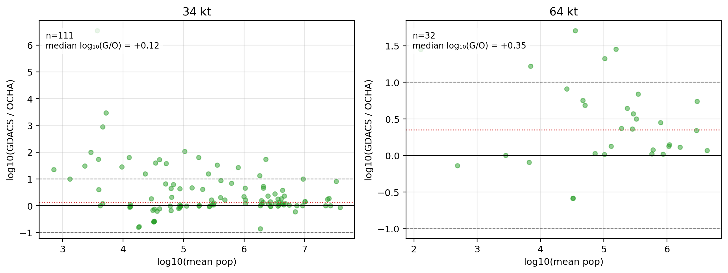
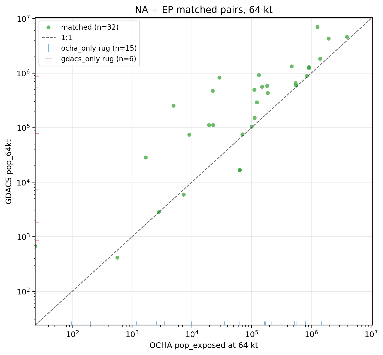
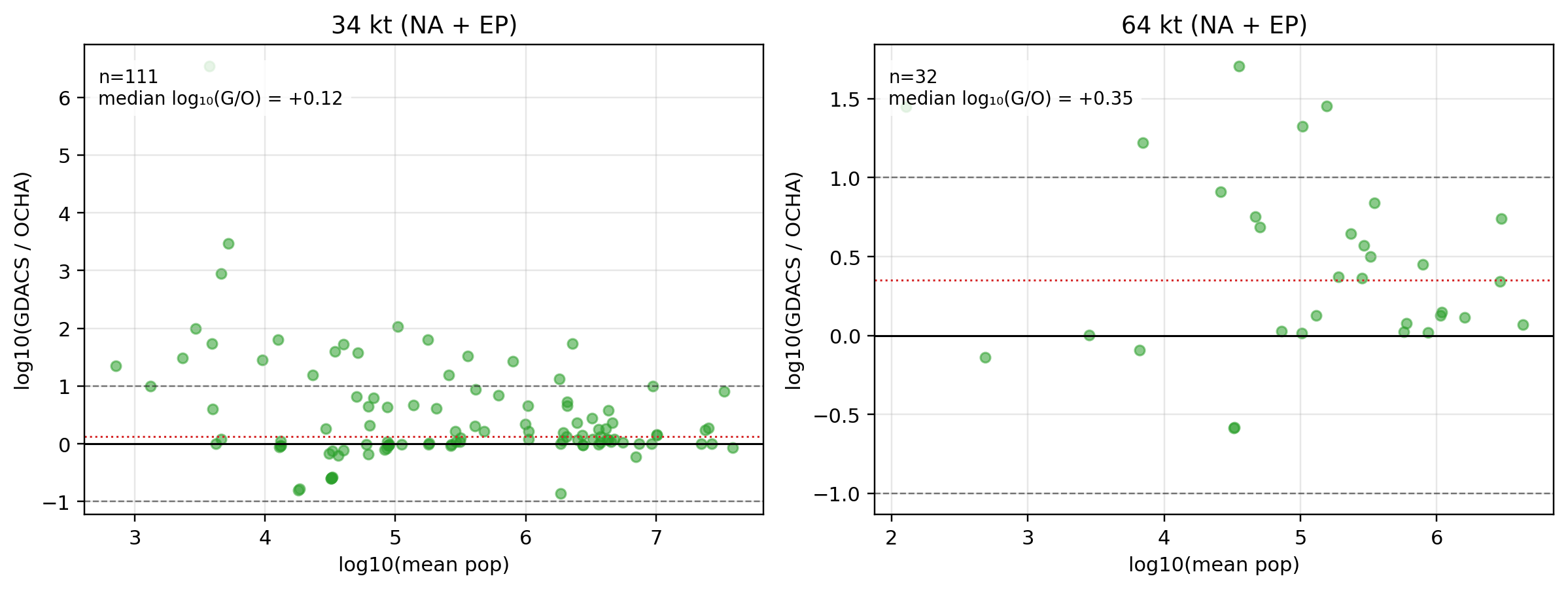
These figures match the global bias table exactly, confirming that every matched pair in the GDACS CSV is already within NA or EP. The remaining spread and bias (~33% median over-estimate by GDACS at 34 kt, more at 64 kt) is within-basin methodological disagreement, not cross-basin noise.
12.7.6 Highest-impact unmatched pairs (NA + EP)
The single-dataset pairs within NA and EP are where real methodology disagreement shows up. If OCHA has a high-exposure entry that GDACS did not record, or vice versa, either the storm sits near one methodology’s inclusion threshold (subtropical, post-tropical, rapidly weakening) or one side simply has a coverage bug.
Top 10 NA/EP storm-country pairs OCHA records but GDACS does not, ordered by OCHA pop at 34 kt.
sid
year
basin
iso3
ocha_34
ocha_64
0
2024268N17278
2024
NA
USA
50,372,416
471,114
1
2024274N14328
2024
NA
USA
35,390,324
nan
2
2022266N12294
2022
NA
USA
30,564,772
1,955,740
3
2024274N14328
2024
NA
RUS
26,762,340
nan
4
2022154N21273
2022
NA
USA
8,662,429
nan
5
2022257N16312
2022
NA
DOM
7,454,846
572,229
6
2023265N29284
2023
NA
USA
6,583,228
nan
7
2024268N17278
2024
NA
CUB
4,154,228
nan
8
2022154N21273
2022
NA
CUB
4,048,040
nan
9
2022266N12294
2022
NA
CUB
3,854,278
546,995
The GDACS-only list is mixed, and the followup probe (see appendix) resolved each case. The high-latitude entries (ERIN 2025 to IRL and GBR, PHILIPPE 2023 over CAN) are post-tropical reaches that OCHA’s tropical-phase methodology excludes. Lower-latitude entries (FRANKLIN 2023 over HTI, ERNESTO 2024 over DOM, NADINE 2024 over HND and GTM) are sensitive to polygon shape: OCHA uses an asymmetric quadrant polygon, GDACS uses a symmetric max-radius circle, and the symmetric circle catches countries at the edge of the footprint that the quadrant polygon misses. For ERNESTO specifically, both datasets share PRI and several Leeward Islands; they differ on exactly which Greater Antilles country the corridor clipped, which is a polygon-shape question not a data-availability one.
The OCHA-only list is more diverse in cause. These are major Atlantic storms with very large populations exposed: HELENE 2024 over the US (50M), KIRK 2024 reaching RUS (27M), IAN 2022 over USA (31M), FIONA 2022 over DOM (7.5M). They do not share a single explanation. The appendix documents the three distinct mechanisms we found: (a) Hannah’s pipeline silently skipping buffer39 on fetch timeout (IAN, OPHELIA), (b) GDACS’s own impact endpoint returning null POP_AFFECTED for every iso3 on certain events (FIONA, ALEX, AGATHA), and (c) CSV snapshot freshness (most 2025 storms were post-snapshot). We confirmed these by rebuilding the pipeline with longer timeouts and retries, uploading a v2 table at ds-storm-impact-harmonisation/raw/gdacs/gdacs_historical_adm0_exposure_v2_NOAA.csv. OCHA-methodology questions like KIRK reporting USA and RUS exposure for a storm that actually moved over Europe may be polygon-overshoot from using a symmetric max-radius reconstruction of post-tropical wind radii.
12.8 Summary
The datasets do not measure the same thing, and the comparison reflects that.
Of 553 storm-country pairs active in 2022+ in at least one dataset, only np.int64(111) have both a GDACS and OCHA value at 34 kt, and only np.int64(32) at 64 kt.
The GDACS CSV is basin-restricted to NA and EP. There are zero 2022+ entries for the Western Pacific, Indian Ocean, or Southern Hemisphere. OCHA-only pairs in those basins are out of CSV scope, not a methodology disagreement. This means methodology comparison is only meaningful within NA + EP.
Within NA + EP, GDACS-only pairs split into two groups: high-latitude countries where post-tropical exposure is being recorded (IRL, GBR, CAN) and lower-latitude countries where subtropical or minor systems are being recorded (DOM, HTI, CUB). OCHA’s IBTrACS-based methodology likely excludes both classes; this is a genuine methodology difference.
Within NA + EP, OCHA-only pairs resolve into three distinct sub-causes (documented in the appendix): pipeline buffer39 fetch timeouts, GDACS’s impact endpoint returning null POP_AFFECTED for every iso3 on certain storms, and CSV snapshot freshness. Only the first is a pipeline bug on the GDACS CSV side and is fixed in the v2 rebuild.
Agreement on matched pairs is reasonable at 34 kt (~55% within 2x, ~80% within 10x, log-log r ≈ 0.72) and noisier at 64 kt (~41% within 2x, r ≈ 0.87 but on only 32 points). GDACS runs ~33% higher than OCHA at 34 kt on average and ~2.2x higher at 64 kt.
Any modelling or downstream comparison should inner-join strictly on matched pairs and treat the unmatched groups as separate populations with their own explanations. Imputing zero for the missing side would bias agreement metrics in both directions.
12.9 Appendix: Pipeline internals and rebuild findings
This appendix records what we verified about the GDACS data flow and the pipeline that produced Hannah’s CSV. Keep this read-only; the numbers above were generated against Hannah’s CSV, and claims here explain why those numbers look the way they do.
12.9.1 A.1 GDACS API structure
The GDACS tropical-cyclone API is a small set of endpoints that chain together. The chart below reflects what we verified empirically in this session. All endpoints are on https://www.gdacs.org/gdacsapi/api.
flowchart TD
    A["/events/geteventlist/search<br/>params: eventlist=TC, fromDate, toDate,<br/>alertlevel, source, pageSize, pageNumber"]
    A -->|paginated list of events| B["/events/geteventdata<br/>?eventtype=TC&eventid=..."]
    B -->|properties.episodes[]| C["/events/getepisodedata<br/>?eventtype=TC&eventid=...&episodeid=..."]
    C --> R["properties.impacts[0].resource"]
    R -->|buffer39 URL| D1["Impact JSON (34 kt)"]
    R -->|buffer74 URL| D2["Impact JSON (64 kt)"]
    R -->|timeline URL| D3["Timeline JSON<br/>per-advisory snapshots"]
    D1 --> E["datums[] array"]
    D2 --> E
    E -->|alias='country'| F1["ADM0 rows<br/>ISO_3DIGIT, CNTRY_NAME,<br/>POP_AFFECTED"]
    E -->|alias='alert'| F2["ADM1 rows<br/>FIPS_ADMIN, GMI_ADMIN,<br/>GMI_CNTRY, POP_AFFECTED"]
    F1 -.->|equivalent at country level<br/>(agree within 1 person rounding)| F2
Key properties verified in this session:
event_id is the GDACS identifier. GDACS does not return IBTrACS SIDs. To attach an SID, the pipeline must join to IBTrACS separately on (season, name).
properties.source on the event-list response is the classification bureau: "NOAA" for Atlantic + Eastern Pacific, "JTWC" for Western Pacific / Indian Ocean / Southern Hemisphere. Hannah’s pipeline filters to NOAA only.
properties.episodes[] is a list of per-advisory snapshots, one per 6-hourly issuance. Each has its own impact URL. See A.4 for what this means for “which episode’s numbers do you actually want.”
buffer39 and buffer74 are named in mph but correspond to 34 kt and 64 kt wind-threshold corridors. See artefacts/01_merge_cerf_exposure/gdacs_endpoint_comparison.md for the reconstruction check that confirmed this.
The country and alert datum groups inside a buffer’s impact JSON are two aggregations of the same data. country is pre-aggregated to ADM0 (one row per iso3). alert is ADM1-level (one row per admin unit) and can be rolled up to country via the GMI_CNTRY column. We verified across 22 KALMAEGI-25 episodes and three production NA storms that the two groups agree at country level to within 1-person rounding. Either is valid; the CSV pipeline uses country, our library code in src/datasets/gdacs.py:215 uses alert.
Buffer39 for major storms (HELENE, IAN) regularly exceeds 30s, so those buffers are silently skipped and the affected iso3 rows end up with pop_34kt = NaN.
Reads alias="country" datum group with ISO_3DIGIT and POP_AFFECTED. Our src/datasets/gdacs.py:get_impact_by_country() reads alias="alert" with GMI_CNTRY. We verified across 22 KALMAEGI-25 episodes and three production NA storms that the two groups return identical country-level numbers to within 1-person rounding; they are redundant slices of the same data, not alternatives.
Reads only the last episode (props["episodes"][-1]). Each episode’s impact is not a cumulative record across the full storm track; it is a snapshot of the union of observed corridor so far plus the forecast cone from that advisory onward. The last episode converges on the observed track because the remaining forecast window is empty. Early episodes can report larger numbers because the forecast cone covered a wider area that later collapsed onto the actual track. For KALMAEGI-25 over PHL: peak was 28.5M at episode 3 of 22; last-episode value 23.0M.
IBTrACS SID join on (season, name) via the internal PostgreSQL storms.ibtracs_storms table. Matches named storms one-to-one; unnamed numeric storms (ONE-C, FOURTEEN-E, etc.) are not matched and produce rows with sid = NaN.
12.9.3 A.3 Verification: GDACS datum groups are equivalent
Checked across three events (FIONA 2022, IAN 2022, HELENE 2024) and 22 cached KALMAEGI-25 episodes. For every (storm, iso3) pair where both alias="country" and alias="alert" had values, they agreed within 1 person. This is rounding in different aggregation pipelines, not a material difference. Either datum group can be used to reproduce the chapter’s numbers.
12.9.4 A.4 Verification: episode impact is per-episode, not cumulative
22-episode trajectory of KALMAEGI-25 buffer39 for each affected country:
iso3
Peak episode
Peak pop
Last episode pop
Last / peak
PHL
3 of 22
28,493,884
23,023,527
0.81
VNM
3 of 22
14,683,360
11,578,200
0.79
THA
9 of 22
7,263,265
2,526,332
0.35
LAO
7 of 22
3,364,733
1,548,365
0.46
KHM
7 of 22
2,796,174
350,147
0.13
No country is monotonically increasing. Each country peaks mid-storm when the forecast cone is widest, then declines as observations resolve the track. Hannah’s CSV records the last-episode value, which is the observed track corridor, not the peak. That is methodologically correct for a post-hoc observational comparison against OCHA’s IBTrACS-based exposure; it would be the wrong choice for reproducing the “what was at risk during the storm” number.
Net effect vs Hannah’s CSV for 2022+ NOAA: 6 additional rows with non-null pop_34kt (IAN USA/CUB/BHS/CYM = 4 rows; OPHELIA 2023 USA/BHS = 2 rows) plus 68 placeholder rows for weak depressions Hannah’s code dropped.
12.9.6 A.6 Three distinct mechanisms behind OCHA-only pairs
Categorising the 95 OCHA-only NA + EP pairs at 34 kt:
Category
Pairs
Cause
Fixable by rerun?
A: SID not in CSV at all
26
Event itself never made it into the CSV
Partly (12 are 2025 storms added later; 4 are subtropical/extratropical OCHA includes but GDACS classifies differently)
B: SID in CSV, this iso3 absent
32
Either GDACS impact did not list this iso3, or it only appeared in the buffer39 response and buffer39 timed out
Sometimes (when buffer39 recovers)
C: CSV has the row, pop_34kt = NaN
37
buffer39 fetch timed out, or GDACS impact returned null POP_AFFECTED for every iso3
Only partly
v2 tested all three. Category C split further: 6 pairs recovered by the timeout + retry fix (IAN, OPHELIA). The remaining ~30 Category-C pairs did not recover because the GDACS impact endpoint itself returns null or 0 for every iso3 on those events (FIONA 2022, ALEX 2022, AGATHA 2022, several others). That is a GDACS-internal issue not resolvable by client-side pipeline changes.
12.9.7 A.7 SID matching is not the failure mode
We considered whether mismatched SID assignment between OCHA and GDACS might be inflating the OCHA-only count. It is not.
match_gdacs_to_ibtracs() in src/datasets/gdacs.py:317 uses (season, name) exact-match. On the 139-event 2022+ NOAA set, zero name-season pairs mapped to multiple SIDs.
10 v2 rows have sid = NaN: all are numerically-named systems (ONE-C-25, FOURTEEN-E-24, etc.) that our matcher deliberately skips via the _UNNAMED_STORMS list in src/datasets/gdacs.py:292. This is correct behavior.
Crossover-name storms (AGATHA 2022 became ALEX 2022) get distinct SIDs in IBTrACS (2022148N13263 for the EP AGATHA track, 2022154N21273 for the NA ALEX track). Both OCHA and GDACS correctly assign these separate SIDs. OCHA has the AGATHA SID with MEX exposure 1.3M at 34 kt; the (AGATHA, MEX) pair classifies as Category C because Hannah’s CSV has the row with pop_34kt = NaN, not because of an SID mismatch.
12.9.8 A.8 The dominant driver of divergence: event-roster scope
Counting unique SIDs in 2022+ NA + EP:
SIDs
v2 (GDACS)
129
OCHA
76
Intersect
63
GDACS-only SIDs
66
OCHA-only SIDs
13
66 storms are in GDACS but not OCHA’s event roster at all. These are mostly subtropical / post-tropical / open-ocean systems that OCHA’s IBTrACS-based pipeline did not produce exposure values for (MARTIN 2022, DANIELLE 2022, EARL 2022, and many unnamed or weakly-named systems). For the 63 storms both track, per-iso3 divergence is the narrower polygon / phase question.
If you want OCHA and GDACS to be compared on the same event roster, the useful hook is not SID matching but event-list intersection. The 13 OCHA-only SIDs are almost all 2025 storms post-dating Hannah’s CSV snapshot; a fresh v2 rebuild would pick up most of them.
12.9.9 A.9 Wind-field method differences for per-iso3 divergence
For the 63 shared storms, per-iso3 divergence is consistent with two previously-documented methodology differences:
Polygon shape: GDACS replaces the four NE/SE/SW/NW quadrant radii with a symmetric circle using max(radii) in all directions (per artefacts/01_merge_cerf_exposure/gdacs_endpoint_comparison.md and the JRC 2016 report). This overstates the affected footprint relative to an asymmetric quadrant polygon, which is the physically realistic shape and likely what OCHA uses.
Phase inclusion: OCHA likely restricts to IBTrACS tropical-phase track points, while GDACS records the entire track including extratropical transitions. This explains ERIN 2025 reaching IRL and GBR in GDACS but only Caribbean iso3s in OCHA, and PHILIPPE 2023 reaching USA and CAN in GDACS but only Leeward Islands in OCHA.
We did not reproduce OCHA’s wind-field reconstruction end-to-end to confirm these hypotheses; the evidence is that every per-iso3 divergence we probed fits one of the two patterns.
12.9.10 A.10 Open questions
Is OCHA’s methodology publicly documented? If yes, settling the polygon-shape and phase-filter hypotheses would be straightforward.
What is driving KIRK 2024’s OCHA footprint over USA (35M) and RUS (27M)? KIRK remained over the Atlantic / Western Europe; the US and Russia numbers suggest either a very wide symmetric-max-radius reconstruction or polygon-projection artifacts. This is an OCHA-side question.
HELENE 2024 buffer39 still times out at 120s with retries. Either a persistent GDACS server issue or an unusually large payload. Could try a 300s+ timeout or contact GDACS.
FIONA 2022 empty data: GDACS’s own impact endpoint returns null POP_AFFECTED for every iso3 at every buffer, at every cached episode. This is unlikely to be recoverable via the public API and would need to be raised with GDACS.