8  CHD vs GDACS vs ADAM: Three-Source Exposure Comparison

We hold three independent estimates of how many people a tropical cyclone exposed — CHD (our NHC-derived figure, the alert pipeline’s number), GDACS (JRC), and ADAM (WFP). This chapter compares all three on a common storm × admin-unit × wind-threshold grid, at the national (adm0) and subnational (adm1) levels. It supersedes the two-way, adm0-only OCHA-vs-GDACS comparison with all three sources, a rigorous five-case zero-vs-NaN basis, and a subnational layer.

The chapter is self-contained: it rebuilds the comparison panels live from the dev database via src/source_exposure (the same build_exposure logic behind the harmonised workbook) and reads the persisted per-storm source diagnostic. It does not depend on any scratch artefacts.

TipKey findings

• Effectively two independent sources — ADAM is a near-duplicate of GDACS (log-correlation 0.94), so the comparison is really CHD vs the GDACS family (Figure 8.7).
• The comparable record is thin — GDACS produces a usable per-country exposure for only ~60 storms (its ~2016–2022 data gaps), so most of the record can’t be compared (Figure 8.1).
• CHD reads about half of GDACS where both find people — median CHD/GDACS ≈ 0.5 on both-positive units; the two also disagree on who is exposed about as often as not (κ ≈ 0) (Figure 8.4).

8.1 TL;DR

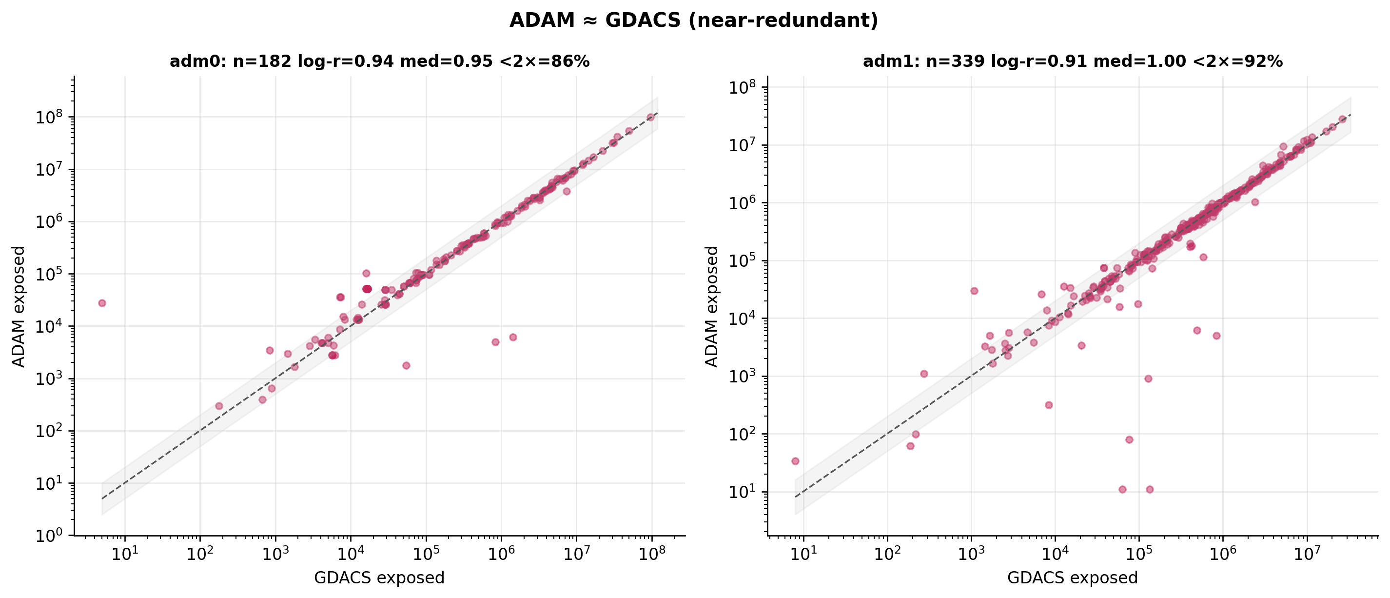
1. It is not a three-way contest. ADAM is a thin near-duplicate of GDACS (log-correlation 0.94, median ratio 0.96, 87% of estimates within 2×). ADAM ingests GDACS upstream and adds almost no independent signal. The real comparison is CHD vs the GDACS family.
2. GDACS produces a usable per-country exposure for only ~60 storms. GDACS exposure has two endpoints — getimpact (per-country) and gettimeline (a single storm-wide total). For its ~2016–2022 era getimpact returns -1 (“not computed”), so for 118 storms GDACS has only a storm total, no per-country breakdown (Matthew, Maria, Harvey among them). Those are data gaps, not zeros, so the per-country comparison is genuinely thin (~60 storms).
3. Where comparable, CHD reads about half of GDACS. On units where both find people CHD runs systematically below GDACS (median CHD/GDACS ≈ 0.5), and this holds at both the country (adm0) and subnational (adm1) level. The sources also disagree on who is exposed about as often as not (κ ≈ 0).

8.2 Method: the GDACS five-case zero-vs-NaN rule

GDACS exposure has two endpoints, and the whole comparison hinges on the difference:

• getimpact — population per country (POP_AFFECTED per iso3). The only source of a per-country breakdown — but it returns -1 (“not computed”) for GDACS’s ~2016–2022 era, which lands in the DB as NULL.
• gettimeline — a single storm-wide total (pop39/pop74: the people inside the whole wind polygon, summed across all areas — not per country). Available back to 2015, so it has a real number even when getimpact is -1 (Matthew 18.3M, Maria 11.6M).

A NULL getimpact value is therefore a per-country DATA GAP, never a true 0. build_exposure fills each (storm, country, threshold) GDACS cell 0 or NaN by a five-case rule — and the storm total is the only signal separating a genuine zero from missing data:

case	situation	fill
1	positive per-country value	the value
2	GDACS computed that threshold (≥1 positive country), this country absent	0 (not in footprint)
3	storm total = 0 (timeline pop39/pop74 = 0)	0 (exposed nobody)
4	per-country -1/NULL, or no per-country value but storm total > 0	NaN (storm total only — no per-country breakdown)
5	storm not tracked, or 50 kt (GDACS has no 50 kt buffer)	NaN

CHD is our own NHC DB, so a missing value is a true 0. All three values are each storm’s final converged estimate — CHD the realized observed-track footprint (latest valid_time per unit, no forecast term added); GDACS and ADAM their final per-episode footprint, which likewise ramps as the footprint establishes then plateaus at the realized value. The comparison is therefore like-for-like: final assessed exposure, with no forecast component on any side. The per-country comparison runs over cells where GDACS is non-NaN (cases 1–3); case-4 storms are recoverable only at the storm-total grain (§5b). Magnitude statistics (log scatter, ratio, Bland–Altman) use both-positive cells only — log(0) is undefined. GDACS carries no 50 kt threshold, so GDACS comparisons use {34, 64} kt.

import sys, os
sys.path.insert(0, "..")
from dotenv import load_dotenv
load_dotenv()

import numpy as np
import pandas as pd
import matplotlib.pyplot as plt
from matplotlib.patches import Circle, Patch

from src.source_exposure import workbook as wb
from src.source_exposure import queries as q
from src.source_exposure import source_diagnostics as sd

plt.rcParams.update({
    "figure.dpi": 120, "savefig.bbox": "tight", "axes.grid": True,
    "grid.alpha": 0.25, "axes.spines.top": False, "axes.spines.right": False,
    "font.size": 10, "axes.titlesize": 12, "axes.titleweight": "bold",
    "figure.facecolor": "white",
})

# ── source bookkeeping ───────────────────────────────────────────────────
SOURCES = ("chd", "gdacs", "adam")
COL = {"chd": "chd_exposure", "gdacs": "gdacs_exposure", "adam": "adam_exposure"}
LABEL = {"chd": "CHD", "gdacs": "GDACS", "adam": "ADAM"}
COLOR = {"chd": "#1b6ca8", "gdacs": "#e07b39", "adam": "#3a9b6e"}
PAIRS = (("chd", "gdacs"), ("chd", "adam"), ("gdacs", "adam"))


def thresholds_for(a, b):
    return (34, 64) if "gdacs" in (a, b) else (34, 50, 64)


def restrict_kt(df, a, b):
    return df[df["wind_speed_kt"].isin(thresholds_for(a, b))]


def overlap(df, a, b):
    d = restrict_kt(df, a, b)
    return d[d[COL[a]].notna() & d[COL[b]].notna()]


def both_positive(df, a, b):
    d = overlap(df, a, b)
    return d[(d[COL[a]] > 0) & (d[COL[b]] > 0)]


def agreement_stats(df, a, b):
    ca, cb = COL[a], COL[b]
    ov = overlap(df, a, b)
    va, vb = ov[ca].to_numpy(float), ov[cb].to_numpy(float)
    bp = (va > 0) & (vb > 0)
    out = {"pair": f"{LABEL[a]} vs {LABEL[b]}", "a": a, "b": b,
           "n_overlap": len(ov), "n_both_pos": int(bp.sum()),
           "n_a_pos_b_zero": int(((va > 0) & (vb == 0)).sum()),
           "n_b_pos_a_zero": int(((va == 0) & (vb > 0)).sum()),
           "n_both_zero": int(((va == 0) & (vb == 0)).sum())}
    if bp.sum() >= 3:
        la, lb = np.log10(va[bp]), np.log10(vb[bp])
        out["pearson_log"] = float(np.corrcoef(la, lb)[0, 1])
        from scipy.stats import spearmanr
        out["spearman"] = float(spearmanr(va[bp], vb[bp]).statistic)
        logr = np.log10(va[bp] / vb[bp])
        out["median_ratio"] = float(np.median(va[bp] / vb[bp]))
        out["pct_within_2x"] = float(np.mean(np.abs(logr) <= np.log10(2)) * 100)
        out["pct_within_10x"] = float(np.mean(np.abs(logr) <= 1.0) * 100)
        out["ba_bias"] = float(np.mean(logr))
        out["ba_sd"] = float(np.std(logr, ddof=1))
        out["ba_lo"] = out["ba_bias"] - 1.96 * out["ba_sd"]
        out["ba_hi"] = out["ba_bias"] + 1.96 * out["ba_sd"]
    else:
        for k in ("pearson_log", "spearman", "median_ratio", "pct_within_2x",
                  "pct_within_10x", "ba_bias", "ba_sd", "ba_lo", "ba_hi"):
            out[k] = float("nan")
    return out


def human(n):
    if n is None or (isinstance(n, float) and np.isnan(n)):
        return "n/a"
    for div, suf in ((1e9, "B"), (1e6, "M"), (1e3, "k")):
        if abs(n) >= div:
            return f"{n / div:.1f}{suf}"
    return f"{n:.0f}"


# ── build the comparison data once (live from the dev DB) ─────────────────
eng = q.get_engine("dev")
aids = q.all_nhc_storms(eng, wb.MIN_SEASON, wb.MAX_SEASON)["atcf_id"].tolist()
chd_rep, gd_rep, ad_rep = q.storms_with_source_exposure(eng, aids)
resolve = wb._country_resolver(eng)
panel0 = wb.build_exposure(eng, 0, aids, gd_rep, ad_rep, resolve)
panel1 = wb.build_exposure(eng, 1, aids, gd_rep, ad_rep, resolve)

# storm roster (presence denominator: all 939 NHC storms >= 2001)
meta = (q.all_nhc_storms(eng, wb.MIN_SEASON, wb.MAX_SEASON)[
        ["atcf_id", "storm_name", "season", "basin"]])
meta["chd_reported"] = meta.atcf_id.isin(chd_rep)
meta["gdacs_reported"] = meta.atcf_id.isin(gd_rep)
meta["adam_reported"] = meta.atcf_id.isin(ad_rep)

# per-storm comparability from the persisted source diagnostic
HOLDS, ZERO = {"have_exposure"}, {"reported_zero", "served_zero"}


def classify(status):
    if pd.isna(status):
        return "never_on_record"
    if status in HOLDS:
        return "holds_exposure"
    if status in ZERO:
        return "reported_zero"
    return "data_gap"


diag = sd.load_status()
comp = meta.merge(diag, on="atcf_id", how="left")
comp["gdacs_class"] = comp["gdacs_status"].map(classify)
comp["adam_class"] = comp["adam_status"].map(classify)
GCLASS = comp.set_index("atcf_id")["gdacs_class"]

# GDACS five-case STATE per storm (authoritative — uses the timeline storm total,
# unlike the persisted diagnostic CSV which predates the fix and mislabels the
# -1 storms as "have_exposure"):
gd_computed = set(s for s, _ in q.gdacs_computed_thresholds(eng, aids))   # >=1 positive per-country
tlt = q.load_timeline_totals()                                            # storm totals (pop39/pop74 max)

def gdacs_state(sid):
    if sid in gd_computed:
        return "computed"                 # case 1/2: real per-country footprint
    if sid in tlt.index and pd.notna(tlt.loc[sid, "timeline_pop39_max"]):
        t39, t74 = tlt.loc[sid, "timeline_pop39_max"], tlt.loc[sid, "timeline_pop74_max"]
        return "genuine_zero" if (t39 == 0 and t74 == 0) else "missing"
    return "not_tracked"                  # GDACS never saw the storm

comp["gdacs_state"] = comp["atcf_id"].map(gdacs_state)
STATE = comp.set_index("atcf_id")["gdacs_state"]

8.3 0. How much GDACS exposure is actually comparable?

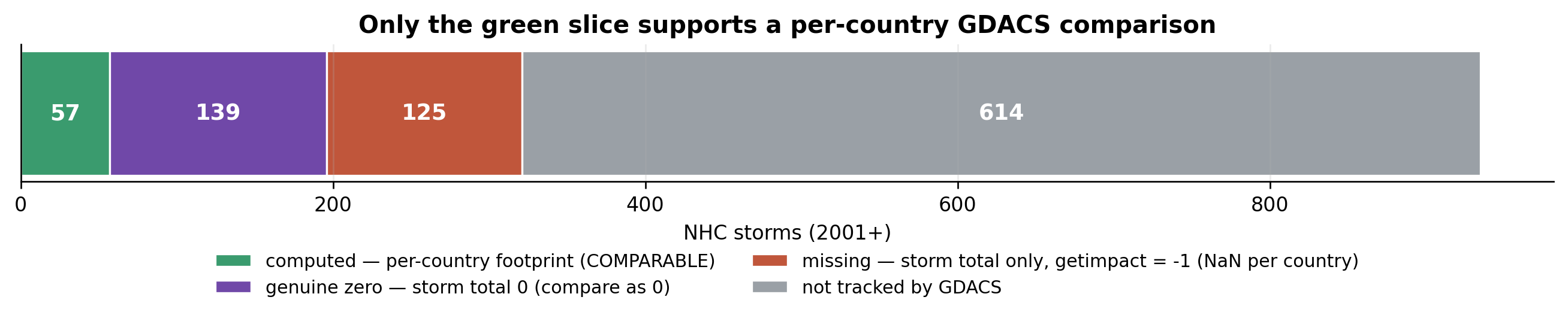
GDACS only produces a usable per-country exposure (its getimpact footprint) for a minority of the storms it tracks. Classifying every NHC storm by its GDACS five-case state makes the comparable slice explicit:

ST_ORDER = ["computed", "genuine_zero", "missing", "not_tracked"]
ST_COL = {"computed": "#3a9b6e", "genuine_zero": "#7048a8",
          "missing": "#c0563b", "not_tracked": "#9aa0a6"}
ST_LAB = {"computed": "computed — per-country footprint (COMPARABLE)",
          "genuine_zero": "genuine zero — storm total 0 (compare as 0)",
          "missing": "missing — storm total only, getimpact = -1 (NaN per country)",
          "not_tracked": "not tracked by GDACS"}
vc = comp["gdacs_state"].value_counts()
fig, ax = plt.subplots(figsize=(11, 2.8))
left = 0
for k in ST_ORDER:
    v = int(vc.get(k, 0))
    if not v:
        continue
    ax.barh(0, v, left=left, color=ST_COL[k], edgecolor="white", label=ST_LAB[k])
    ax.text(left + v / 2, 0, str(v), ha="center", va="center", fontsize=11,
            fontweight="bold", color="white")
    left += v
ax.set_yticks([]); ax.set_xlabel("NHC storms (2001+)"); ax.grid(axis="y", alpha=0)
ax.legend(loc="upper center", bbox_to_anchor=(0.5, -0.4), ncol=2, frameon=False,
          fontsize=9)
ax.set_title("Only the green slice supports a per-country GDACS comparison")
fig.tight_layout()
plt.show()

Figure 8.1: GDACS five-case state per NHC storm (2001+). Only computed storms (≥1 positive per-country value) support a per-country comparison; genuine zero storms (storm total = 0) compare as 0; missing storms have a real gettimeline storm total but no per-country breakdown (getimpact = -1, GDACS’s ~2016-2022 era) so they are NaN per country; not tracked storms GDACS never saw.

Of the storms GDACS tracks, only 60 have a real per-country footprint (cases 1–2). 135 are genuine zeros (storm total = 0, comparable as a 0). 119 are data gaps — GDACS has a gettimeline storm total but never computed the per-country breakdown (getimpact = -1), so they are NaN per country and recoverable only as a storm total (§5b). Maria, Harvey and Matthew sit here — large, real storms GDACS did size storm-wide (12M / 0.5M / 18M), just never broke down by country. So the per-country comparison is genuinely thin (~60 storms): a -1 is a missing per-country breakdown, not a zero.

8.4 1. Coverage — who reports which storms

chd = set(meta.loc[meta.chd_reported, "atcf_id"])
gd = set(meta.loc[meta.gdacs_reported, "atcf_id"])
ad = set(meta.loc[meta.adam_reported, "atcf_id"])
n_chd, n_gd, n_ad = len(chd), len(gd), len(ad)
cell = {"CHD only": len(chd - gd - ad), "CHD&GDACS": len((chd & gd) - ad),
        "all three": len(chd & gd & ad), "CHD&ADAM": len((chd & ad) - gd),
        "GDACS&ADAM not CHD": len((gd & ad) - chd),
        "GDACS only": len(gd - chd - ad), "ADAM only": len(ad - chd - gd)}

fig, (axv, axb) = plt.subplots(1, 2, figsize=(13.5, 6.0),
                               gridspec_kw={"width_ratios": [1.0, 1.05]})
axv.set_aspect("equal"); axv.axis("off")
scale = 0.40 / np.sqrt(n_chd)
R = {k: np.sqrt(v) * scale for k, v in (("chd", n_chd), ("gd", n_gd), ("ad", n_ad))}
cx, cy = 0.52, 0.5
gx, gy = cx - (R["chd"] - R["gd"]) * 0.5, cy - (R["chd"] - R["gd"]) * 0.22
# ADAM links to GDACS events but computes exposure independently, so it pokes
# outside the (thin) GDACS positive-per-country set wherever GDACS is a genuine
# zero or a per-country data gap (-1) yet ADAM found people.
axc = (gx + R["gd"] * 0.50, gy + R["gd"] * 0.22)
n_ad_not_gd = len(ad - gd)
axv.add_patch(Circle((cx, cy), R["chd"], facecolor=COLOR["chd"], alpha=0.15,
                     edgecolor=COLOR["chd"], lw=2.4))
axv.add_patch(Circle((gx, gy), R["gd"], facecolor=COLOR["gdacs"], alpha=0.30,
                     edgecolor=COLOR["gdacs"], lw=2.2))
axv.add_patch(Circle(axc, R["ad"], facecolor=COLOR["adam"], alpha=0.45,
                     edgecolor=COLOR["adam"], lw=2.2))
axv.text(cx + R["chd"] * 0.3, cy + R["chd"] * 0.74, f"CHD\n{n_chd}", ha="center",
         va="center", fontsize=12.5, fontweight="bold", color=COLOR["chd"])
axv.text(gx - R["gd"] * 0.34, gy - R["gd"] * 0.5, f"GDACS\n{n_gd}", ha="center",
         va="center", fontsize=10.5, fontweight="bold", color=COLOR["gdacs"])
axv.text(axc[0] + R["ad"] * 0.45, axc[1] + R["ad"] * 0.5, f"ADAM\n{n_ad}",
         ha="center", va="center", fontsize=10, fontweight="bold", color=COLOR["adam"])
# annotate the ADAM sliver outside the GDACS positive-per-country set
axv.annotate(f"{n_ad_not_gd} ADAM storms outside the\nGDACS positive set "
             "(GDACS zero\nor data gap; ADAM found people)",
             xy=(axc[0] + R["ad"] * 0.95, axc[1] - R["ad"] * 0.2),
             xytext=(0.80, 0.16), fontsize=7.5, color=COLOR["adam"], ha="center",
             arrowprops=dict(arrowstyle="->", color=COLOR["adam"], lw=1))
axv.set_xlim(0.02, 0.98); axv.set_ylim(0.02, 0.98)
axv.set_title("Storms with a positive per-country exposure\n"
              f"(CHD {n_chd}, GDACS {n_gd}, ADAM {n_ad}; "
              f"{n_ad_not_gd} ADAM outside the GDACS-positive set)", fontsize=10.5)
order = ["CHD only", "CHD&GDACS", "all three", "CHD&ADAM",
         "GDACS&ADAM not CHD", "GDACS only", "ADAM only"]
cmap = {"CHD only": COLOR["chd"], "CHD&GDACS": "#9a6a3a", "all three": "#7a4a8a",
        "CHD&ADAM": "#2a7a8a", "GDACS&ADAM not CHD": COLOR["gdacs"],
        "GDACS only": COLOR["gdacs"], "ADAM only": COLOR["adam"]}
vals = [cell[k] for k in order]; yp = np.arange(len(order))
axb.barh(yp, vals, color=[cmap[k] for k in order], alpha=0.85, edgecolor="white")
axb.set_yticks(yp); axb.set_yticklabels(order, fontsize=9.5); axb.invert_yaxis()
for y, v in zip(yp, vals):
    axb.text(v + max(vals) * 0.012, y, str(v), va="center", fontsize=10, fontweight="bold")
axb.set_xlabel("NHC storms (2001–2026)"); axb.set_xlim(0, max(vals) * 1.14)
axb.set_title(f"Exclusive coverage cells (of {len(meta)} storms)", fontsize=11)
axb.grid(axis="y", alpha=0)
fig.tight_layout()
plt.show()

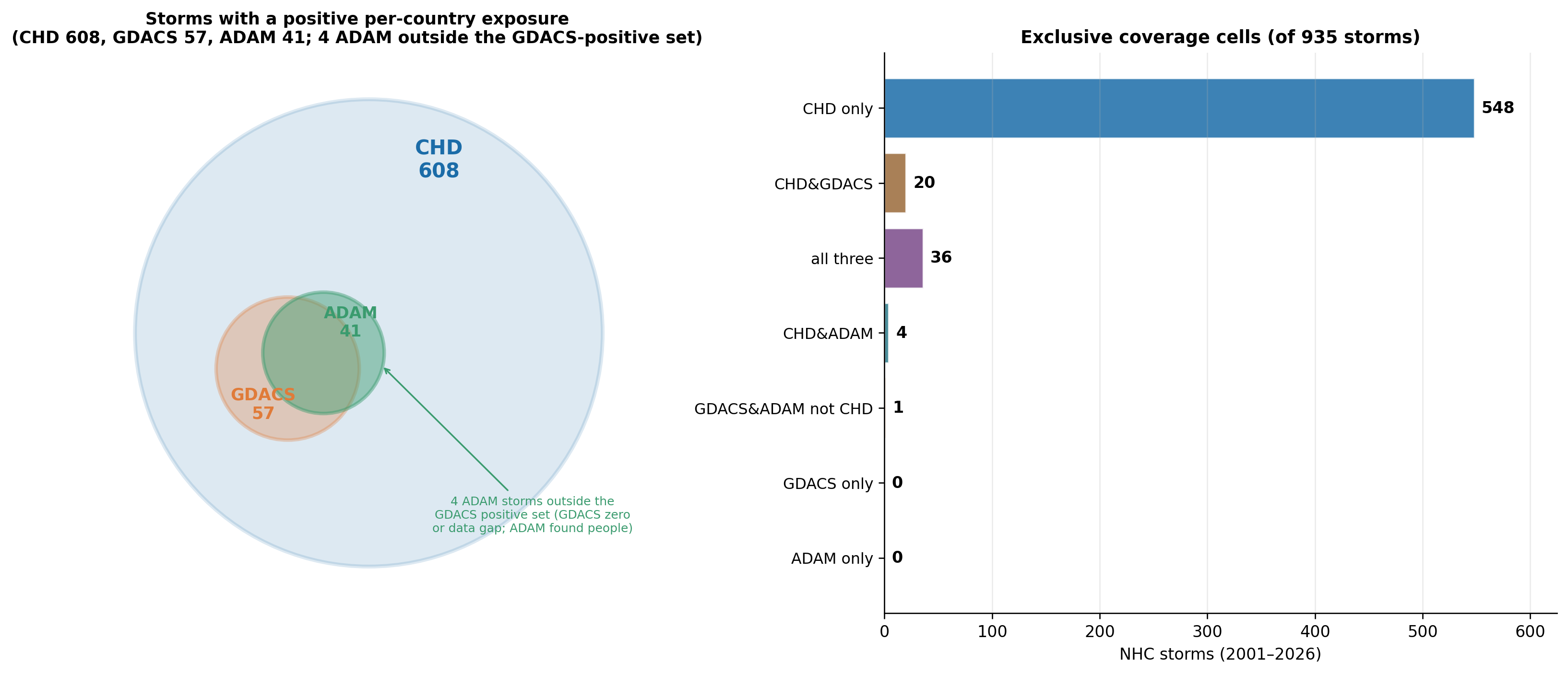
Figure 8.2: Storm-level coverage — counting which storms each source produces a POSITIVE per-country exposure number for (GDACS case 1/2 only). CHD 611, GDACS 60, ADAM 44 of 939 storms. GDACS’s count is small because its per-country footprint is missing (getimpact = -1) for ~116 storms; ADAM, which computes exposure independently, sits partly outside that thin GDACS-positive set. The bar gives the exact 7-cell breakdown.

seasons = sorted(meta.season.unique())
per = {s: [int(meta[(meta.season == ss) & meta[f"{s}_reported"]].shape[0])
           for ss in seasons] for s in SOURCES}
fig, ax = plt.subplots(figsize=(12, 4.8))
x = np.array(seasons); bw = 0.78 / 3
for i, s in enumerate(SOURCES):
    ax.bar(x + (i - 1) * bw, per[s], bw, label=LABEL[s], color=COLOR[s], alpha=0.9)
ax.set_xlabel("season"); ax.set_ylabel("storms reported")
ax.set_xticks(x); ax.set_xticklabels(x, rotation=90, fontsize=8)
ax.legend(title="source", frameon=False)
ax.set_title("GDACS (2015+) and ADAM (2023+) only become usable recently")
fig.tight_layout()
plt.show()

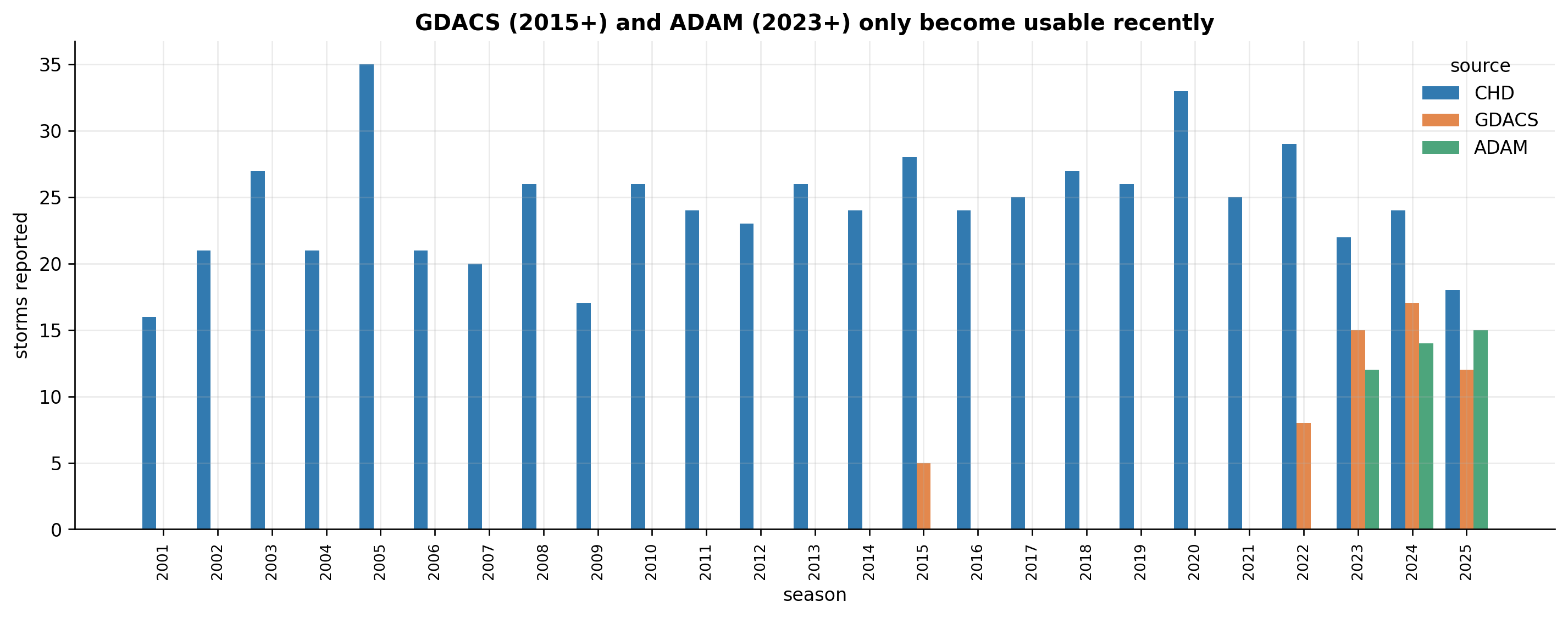
Figure 8.3: Coverage over time. CHD spans the full record; GDACS only switches on in 2015 and ADAM in 2023 — so any historical comparison is impossible, and the headline coverage gap is largely a recency artefact.

The per-country-comparable slice is small and recent: GDACS has a positive per-country footprint for only 60 storms (vs 611 for CHD), almost all 2022+ — both because GDACS/ADAM are recent (2015 / 2023) and because GDACS’s per-country getimpact is -1 for its earlier era. So CHD-vs-GDACS per-country agreement can only be assessed on that thin slice; the rest is recovered, if at all, at the storm-total grain.

8.5 2. Magnitude — where both report a positive number (adm0)

ks = [34, 50, 64]
fig, axes = plt.subplots(3, 3, figsize=(12, 11))
for i, (a, b) in enumerate(PAIRS):
    for j, k in enumerate(ks):
        ax = axes[i, j]
        if k not in thresholds_for(a, b):
            ax.text(0.5, 0.5, f"{LABEL[b] if 'gdacs' in (a,b) else ''}\nno 50 kt",
                    ha="center", va="center", transform=ax.transAxes,
                    fontsize=9, color="#999"); ax.set_xticks([]); ax.set_yticks([])
            continue
        d = both_positive(panel0[panel0.wind_speed_kt == k], a, b)
        xv, yv = d[COL[a]], d[COL[b]]
        ax.scatter(xv, yv, s=14, alpha=0.5, color=COLOR[a] if a != "gdacs" else COLOR["gdacs"])
        if len(d):
            lim = [max(1, min(xv.min(), yv.min())), max(xv.max(), yv.max()) * 1.2]
            ax.plot(lim, lim, "--", color="#555", lw=1)
            ax.fill_between(lim, [v / 2 for v in lim], [v * 2 for v in lim],
                            color="#bbb", alpha=0.15)
            ax.set_xscale("log"); ax.set_yscale("log")
            r = np.corrcoef(np.log10(xv), np.log10(yv))[0, 1] if len(d) > 2 else np.nan
            ax.set_title(f"{LABEL[a]} vs {LABEL[b]} · {k} kt\n"
                         f"n={len(d)} log-r={r:.2f} med={np.median(xv/yv):.2f}",
                         fontsize=9)
        ax.set_xlabel(f"{LABEL[a]} exposed"); ax.set_ylabel(f"{LABEL[b]} exposed")
fig.suptitle("adm0 magnitude agreement (both-positive)", fontsize=13,
             fontweight="bold", y=1.0)
fig.tight_layout()
plt.show()

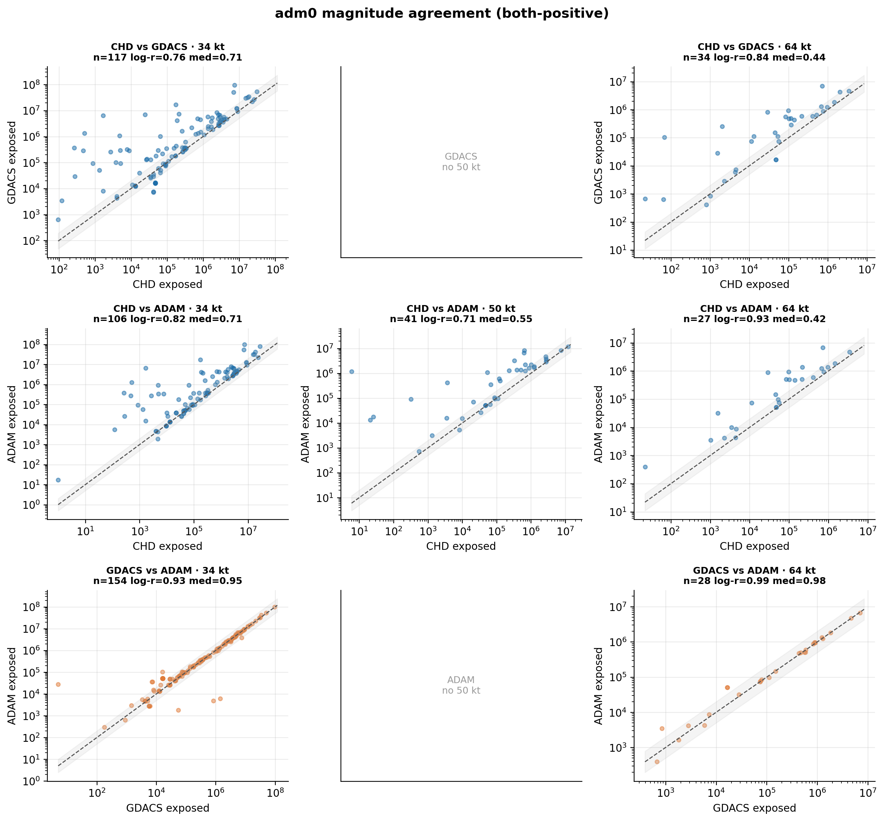
Figure 8.4: Log-log scatter of adm0 exposure on both-positive rows, per source pair × wind threshold (GDACS pairs have no 50 kt). Dashed identity line, shaded within-2× band. GDACS-vs-ADAM hugs the line; CHD disagrees with both, running systematically low.

fig, ax = plt.subplots(figsize=(9, 5))
data, labs, cols = [], [], []
for a, b in PAIRS:
    d = both_positive(panel0, a, b)
    data.append(np.log10(d[COL[a]] / d[COL[b]]))
    labs.append(f"{LABEL[a]}/{LABEL[b]}\n(n={len(d)})"); cols.append(COLOR[a])
parts = ax.violinplot(data, showmedians=True, vert=False)
for pc, c in zip(parts["bodies"], cols):
    pc.set_facecolor(c); pc.set_alpha(0.5)
for r, ls in [(0, "-"), (np.log10(2), ":"), (-np.log10(2), ":")]:
    ax.axvline(r, color="#888", ls=ls, lw=1)
ax.set_yticks(range(1, len(labs) + 1)); ax.set_yticklabels(labs)
ax.set_xlabel("log10(ratio a/b)  —  0 = parity, ±0.3 = within 2×")
ax.set_title("Exposure ratio distributions (adm0, both-positive)")
fig.tight_layout()
plt.show()

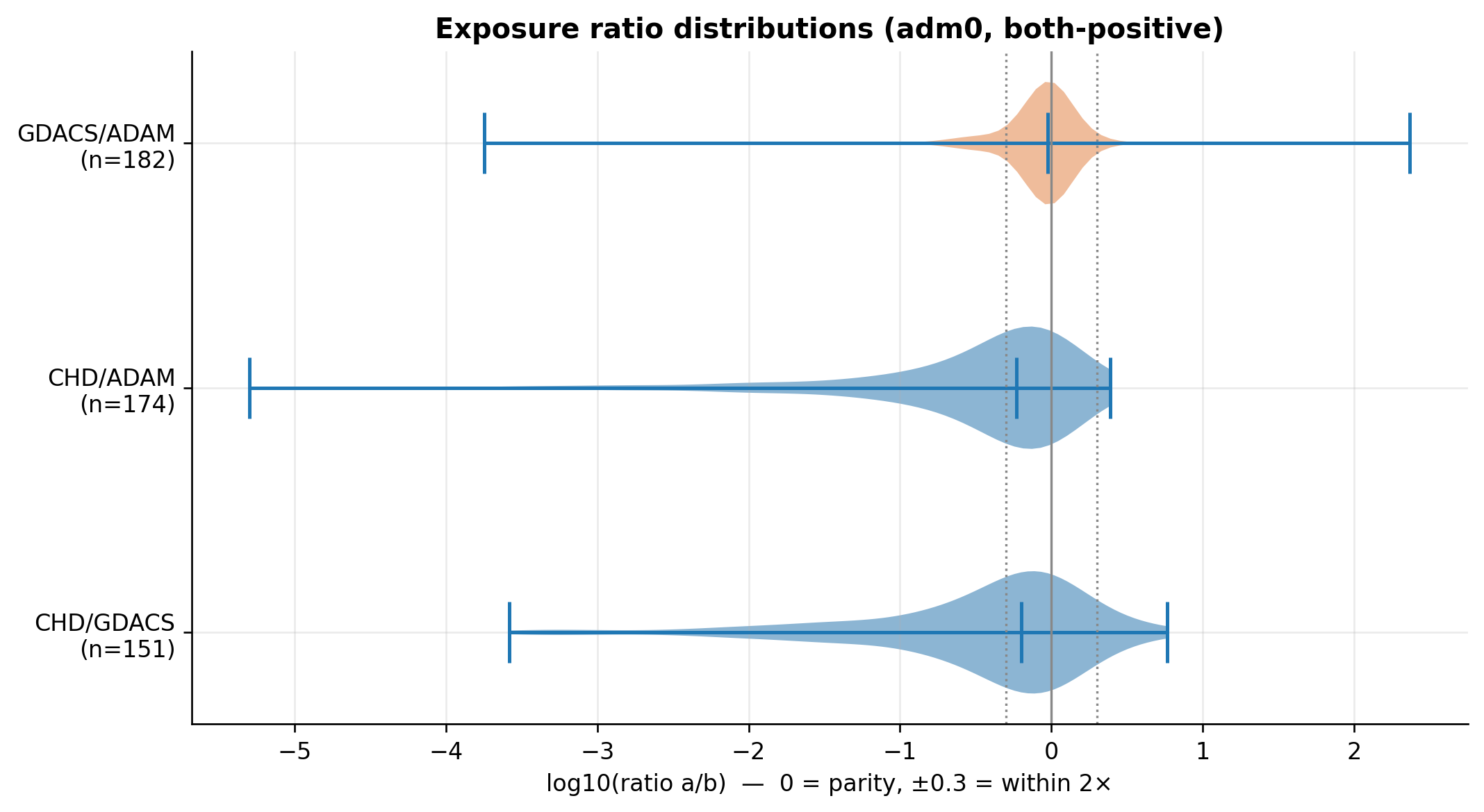
Figure 8.5: Distribution of log10 exposure ratio (a/b) per pair on both-positive adm0 rows. Reference lines at ratio 0.5, 1, 2. CHD pairs sit well below parity (CHD reports fewer people); GDACS-vs-ADAM peaks tightly at 1.0.

Where both sources report a positive adm0 exposure, GDACS and ADAM agree almost perfectly (log-r 0.94, median 0.96, 87% within 2×, near-zero bias). CHD disagrees with both, in the same direction — it reports about half as many people (median ratios 0.58 / 0.57), with wide, heteroscedastic scatter. So two sources are near-clones and CHD is the systematic low outlier.

8.6 3. Bland–Altman and the agreement table

fig, axes = plt.subplots(1, 3, figsize=(14, 4.4))
for ax, (a, b) in zip(axes, PAIRS):
    d = both_positive(panel0, a, b)
    m = (np.log10(d[COL[a]]) + np.log10(d[COL[b]])) / 2
    diff = np.log10(d[COL[a]] / d[COL[b]])
    s = agreement_stats(panel0, a, b)
    ax.scatter(m, diff, s=14, alpha=0.5, color=COLOR[a])
    ax.axhline(s["ba_bias"], color="#c0563b", lw=1.4)
    for v in (s["ba_lo"], s["ba_hi"]):
        ax.axhline(v, color="#c0563b", ls="--", lw=1)
    ax.axhline(0, color="#555", lw=0.8)
    ax.set_title(f"{LABEL[a]} vs {LABEL[b]}\nbias={s['ba_bias']:.2f} "
                 f"LoA[{s['ba_lo']:.2f},{s['ba_hi']:.2f}]", fontsize=9.5)
    ax.set_xlabel("mean log10 exposure"); ax.set_ylabel(f"log10({LABEL[a]}/{LABEL[b]})")
fig.tight_layout()
plt.show()

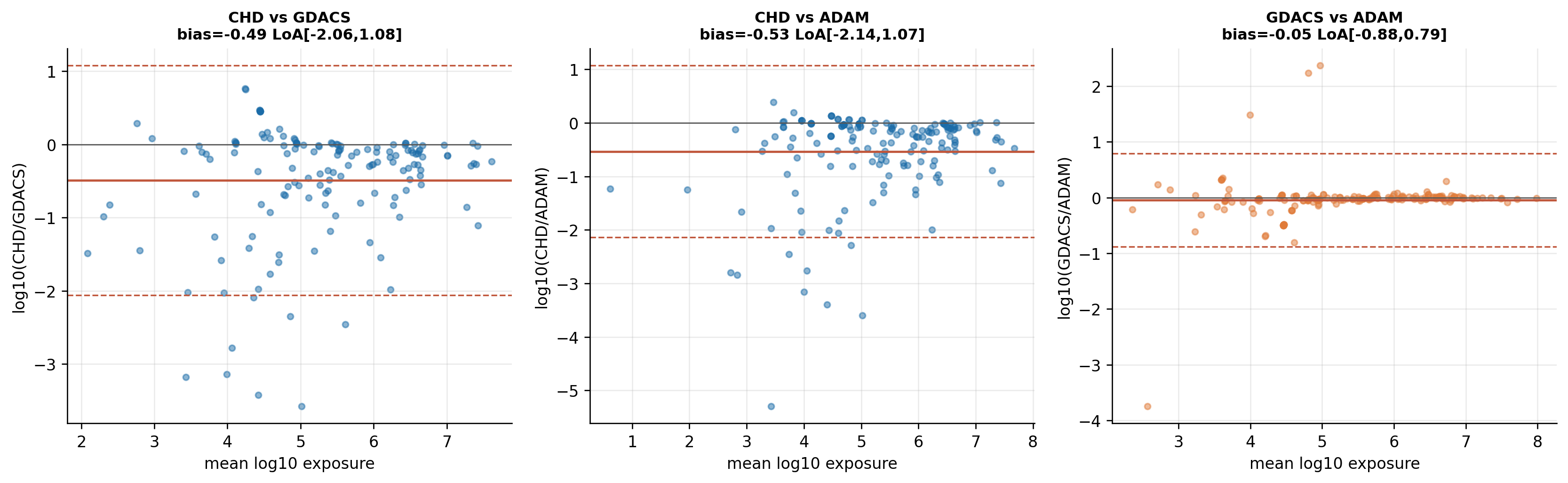
Figure 8.6: Bland–Altman plots (both-positive adm0). CHD vs GDACS and CHD vs ADAM show a large negative bias and limits of agreement spanning ~±2 decades; GDACS vs ADAM is tight and near-unbiased.

rows = []
for a, b in PAIRS:
    s = agreement_stats(panel0, a, b)
    rows.append({"pair": s["pair"], "both-pos n": s["n_both_pos"],
                 "a>0,b=0": s["n_a_pos_b_zero"], "b>0,a=0": s["n_b_pos_a_zero"],
                 "log-r": round(s["pearson_log"], 3),
                 "median a/b": round(s["median_ratio"], 2),
                 "within 2×": f"{s['pct_within_2x']:.0f}%",
                 "BA bias": round(s["ba_bias"], 2)})
pd.DataFrame(rows).set_index("pair")

Table 8.1

	both-pos n	a>0,b=0	b>0,a=0	log-r	median a/b	within 2×	BA bias
pair
CHD vs GDACS	151	38	104	0.791	0.63	52%	-0.49
CHD vs ADAM	174	11	100	0.801	0.59	56%	-0.53
GDACS vs ADAM	182	10	26	0.936	0.95	86%	-0.05

8.7 4. Is ADAM just GDACS?

fig, axes = plt.subplots(1, 2, figsize=(12, 5.2))
for ax, (panel, lvl) in zip(axes, ((panel0, "adm0"), (panel1, "adm1"))):
    d = both_positive(panel, "gdacs", "adam")
    ax.scatter(d["gdacs_exposure"], d["adam_exposure"], s=16, alpha=0.5,
               color="#c2255c")
    if len(d):
        lim = [max(1, d[["gdacs_exposure", "adam_exposure"]].min().min()),
               d[["gdacs_exposure", "adam_exposure"]].max().max() * 1.2]
        ax.plot(lim, lim, "--", color="#555", lw=1)
        ax.fill_between(lim, [v / 2 for v in lim], [v * 2 for v in lim],
                        color="#bbb", alpha=0.15)
    ax.set_xscale("log"); ax.set_yscale("log")
    s = agreement_stats(panel, "gdacs", "adam")
    ax.set_title(f"{lvl}: n={s['n_both_pos']} log-r={s['pearson_log']:.2f} "
                 f"med={s['median_ratio']:.2f} <2×={s['pct_within_2x']:.0f}%",
                 fontsize=10)
    ax.set_xlabel("GDACS exposed"); ax.set_ylabel("ADAM exposed")
fig.suptitle("ADAM ≈ GDACS (near-redundant)", fontsize=12, fontweight="bold")
fig.tight_layout()
plt.show()

Figure 8.7: GDACS vs ADAM on both-positive rows (adm0 and adm1). Points hug the 1:1 line (adm0 log-r 0.94, adm1 0.91, median ratio ~1.0). ADAM is a re-derivation of GDACS, not independent evidence.

ADAM tracks GDACS one-to-one where they overlap, ingests it upstream, and covers only 56 storms (75% already in GDACS). Treated co-equally with CHD, it contributes essentially no independent signal. GDACS+ADAM should be treated as one source.

8.8 5. The zero-gap — the dominant CHD-vs-GDACS disagreement (adm0)

cells = ["n_both_pos", "n_a_pos_b_zero", "n_b_pos_a_zero", "n_both_zero"]
clab = {"n_both_pos": "both positive", "n_a_pos_b_zero": "A>0, B=0",
        "n_b_pos_a_zero": "B>0, A=0", "n_both_zero": "both 0"}
ccol = {"n_both_pos": "#7048a8", "n_a_pos_b_zero": "#c2255c",
        "n_b_pos_a_zero": "#e8788f", "n_both_zero": "#ced4da"}
fig, ax = plt.subplots(figsize=(9.5, 4.6))
yy = np.arange(len(PAIRS))[::-1]
for y, (a, b) in zip(yy, PAIRS):
    s = agreement_stats(panel0, a, b); left = 0
    for c in cells:
        ax.barh(y, s[c], left=left, height=0.6, color=ccol[c], edgecolor="white")
        if s[c] > 25:
            ax.text(left + s[c] / 2, y, f"{s[c]:,}", va="center", ha="center",
                    fontsize=8.5, color="white" if c != "n_both_zero" else "#333")
        left += s[c]
ax.set_yticks(yy); ax.set_yticklabels([f"{LABEL[a]} (A) vs {LABEL[b]} (B)" for a, b in PAIRS])
ax.set_xlabel("matched adm0 cells"); ax.grid(axis="y", visible=False)
ax.legend(handles=[Patch(facecolor=ccol[c], label=clab[c]) for c in cells],
          loc="lower right", fontsize=8.5, ncol=2)
ax.set_title("adm0 overlap: both-positive plus a modest defensible zero-gap")
fig.tight_layout()
plt.show()

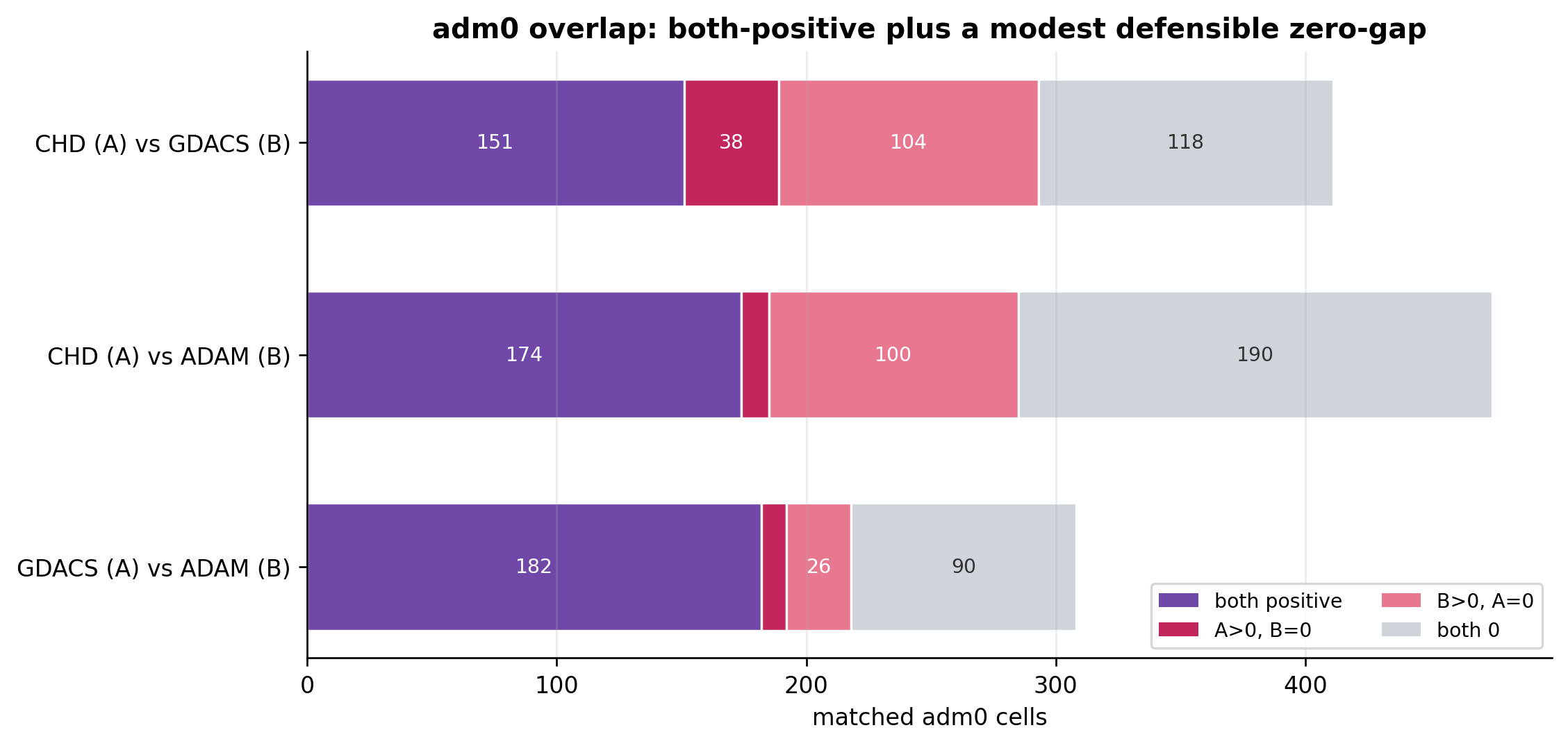
Figure 8.8: Four-cell split of the adm0 overlap per pair (GDACS cells are 0-vs-NaN per the five-case rule). For CHD vs GDACS the defensible zero-gap (CHD>0, GDACS true 0) is modest relative to the both-positive set, because GDACS’s -1 ‘not computed’ values are held out as NaN rather than counted as 0.

ov = overlap(panel0, "chd", "gdacs")
chd_only = ov[(ov.chd_exposure > 0) & (ov.gdacs_exposure == 0)].nlargest(12, "chd_exposure")
gd_only = ov[(ov.gdacs_exposure > 0) & (ov.chd_exposure == 0)].nlargest(12, "gdacs_exposure")
fig, axes = plt.subplots(1, 2, figsize=(13.5, 5.6))
for ax, dfp, vc, color, title in (
        (axes[0], chd_only, "chd_exposure", COLOR["chd"], "CHD>0 · GDACS=0"),
        (axes[1], gd_only, "gdacs_exposure", COLOR["gdacs"], "GDACS>0 · CHD=0")):
    dfp = dfp.iloc[::-1]; yy = np.arange(len(dfp))
    ax.barh(yy, dfp[vc] / 1e6, color=color, edgecolor="white")
    ax.set_yticks(yy)
    ax.set_yticklabels([f"{r.storm_name.title()} {int(r.season)} — {r.admin_name}"
                        for r in dfp.itertuples()], fontsize=8)
    for i, v in enumerate(dfp[vc].to_numpy()):
        ax.text(v / 1e6, i, f" {human(v)}", va="center", fontsize=8)
    ax.set_xlabel("population exposed (M)"); ax.set_title(title, color=color)
    ax.grid(axis="y", visible=False); ax.margins(x=0.18)
fig.tight_layout()
plt.show()

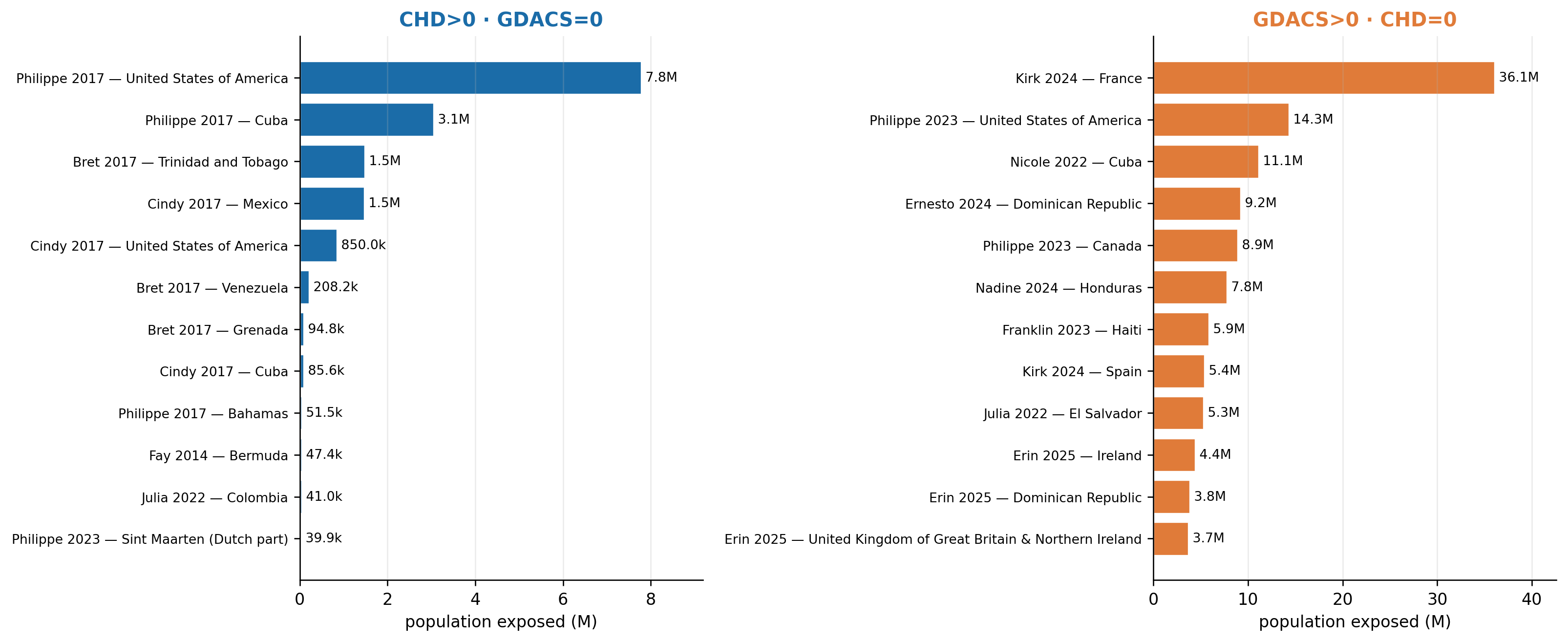
Figure 8.9: Largest adm0 CHD-vs-GDACS zero-gaps, both directions, over the comparable (non-NaN) set. CHD finds exposure where GDACS computed the storm but placed no population in this country at this threshold — mostly 34 kt clips of large, dense countries.

Of the 418 CHD-vs-GDACS adm0 comparable cells (both non-NaN), 153 are both-positive, 38 are CHD-positive while GDACS is a true 0 (case 2/3 — GDACS computed the storm but didn’t place this country in its footprint), and 109 the reverse (GDACS positive, CHD a true 0). These are defensible zeros — GDACS’s -1 “not computed” values are excluded as NaN, never counted as 0.

8.8.1 5b. The missing storms — recoverable only as a storm total

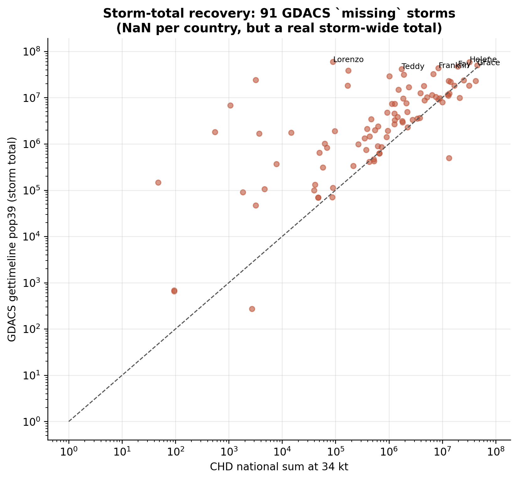
The 119 missing storms are GDACS’s per-country data gaps: getimpact returned -1, so they are NaN per country and absent from §2–§5. But GDACS did size them storm-wide via gettimeline. At that grain they are still comparable — CHD’s national sum vs GDACS’s storm total:

miss = comp[comp.gdacs_state == "missing"].atcf_id
chd_tot = (panel0[(panel0.atcf_id.isin(miss)) & (panel0.wind_speed_kt == 34)]
           .groupby("atcf_id").agg(name=("storm_name", "first"),
            chd=("chd_exposure", "sum")))
chd_tot["gd_timeline"] = chd_tot.index.map(
    lambda s: tlt.loc[s, "timeline_pop39_max"] if s in tlt.index else np.nan)
d = chd_tot.dropna(subset=["gd_timeline"])
d = d[(d.chd > 0) & (d.gd_timeline > 0)]
fig, ax = plt.subplots(figsize=(7, 6.5))
ax.scatter(d.chd, d.gd_timeline, s=24, alpha=0.6, color="#c0563b")
lim = max(d.chd.max(), d.gd_timeline.max()) * 1.3
ax.plot([1, lim], [1, lim], "--", color="#555", lw=1)
ax.set_xscale("log"); ax.set_yscale("log")
ax.set_xlabel("CHD national sum at 34 kt")
ax.set_ylabel("GDACS gettimeline pop39 (storm total)")
for s, r in d.nlargest(6, "gd_timeline").iterrows():
    ax.annotate(r["name"].title(), (r.chd, r.gd_timeline), fontsize=7.5)
ax.set_title(f"Storm-total recovery: {len(d)} GDACS `missing` storms\n"
             "(NaN per country, but a real storm-wide total)")
fig.tight_layout()
plt.show()

Figure 8.10: Storm-total comparison for the GDACS missing storms (per-country = -1, but a real gettimeline total). CHD’s 34 kt national sum vs GDACS’s pop39 storm total. These are dropped entirely from the per-country grid; at the storm grain they are comparable and GDACS’s totals are large and real (Matthew, Maria, …).

So the missing storms are not absent from GDACS — only their per-country breakdown is. A storm-total comparison recovers them. But because the timeline total is storm-wide (not per country), it can never enter the per-country grid — which is exactly why the per-country comparison stays at ~60 storms.

8.9 6. Subnational — the same story, amplified by matching (adm1)

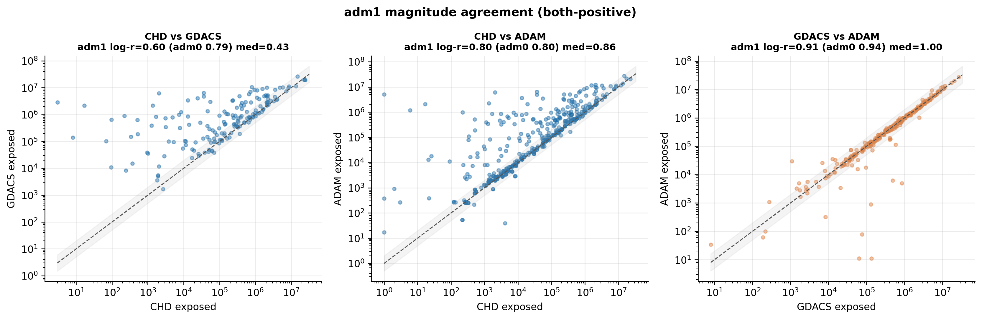
fig, axes = plt.subplots(1, 3, figsize=(14, 4.6))
for ax, (a, b) in zip(axes, PAIRS):
    d = both_positive(panel1, a, b)
    ax.scatter(d[COL[a]], d[COL[b]], s=12, alpha=0.45, color=COLOR[a])
    if len(d):
        lim = [max(1, d[[COL[a], COL[b]]].min().min()),
               d[[COL[a], COL[b]]].max().max() * 1.2]
        ax.plot(lim, lim, "--", color="#555", lw=1)
        ax.fill_between(lim, [v / 2 for v in lim], [v * 2 for v in lim],
                        color="#bbb", alpha=0.15)
    ax.set_xscale("log"); ax.set_yscale("log")
    s0 = agreement_stats(panel0, a, b); s1 = agreement_stats(panel1, a, b)
    ax.set_title(f"{LABEL[a]} vs {LABEL[b]}\nadm1 log-r={s1['pearson_log']:.2f} "
                 f"(adm0 {s0['pearson_log']:.2f}) med={s1['median_ratio']:.2f}",
                 fontsize=9.5)
    ax.set_xlabel(f"{LABEL[a]} exposed"); ax.set_ylabel(f"{LABEL[b]} exposed")
fig.suptitle("adm1 magnitude agreement (both-positive)", fontsize=12, fontweight="bold")
fig.tight_layout()
plt.show()

Figure 8.11: adm1 both-positive scatter per pair (vs the adm0 log-r inline). CHD-vs-GDACS degrades most going subnational (log-r 0.60 vs 0.79, median 0.43); GDACS-vs-ADAM stays tight.

dk = restrict_kt(panel1, "chd", "gdacs")
chdpos = dk[dk.chd_exposure > 0].copy()
chdpos["gstate"] = chdpos.atcf_id.map(STATE)
chdpos = chdpos[chdpos.gstate == "computed"]   # GDACS produced a per-country footprint


def caveat_cat(row):
    gv = row["gdacs_exposure"]
    cav = str(row.get("adm1_caveat") or "")
    gc = ""
    for part in cav.split("|"):
        if part.strip().startswith("GDACS:"):
            gc = part.split(":", 1)[1].strip()
    if pd.notna(gv) and gv > 0:
        return ("both positive", "genuine")
    if pd.notna(gv) and gv == 0:
        return ("GDACS real 0 (zero-gap)", "genuine")
    if "national-only" in gc:
        return ("blank: national-only", "method")
    if "no counterpart" in gc:
        return ("blank: no FM counterpart", "method")
    return ("blank: not listed", "method")


cc = chdpos.apply(caveat_cat, axis=1, result_type="expand")
chdpos = chdpos.assign(cat=cc[0], nature=cc[1])
g = chdpos.groupby("cat").agg(units=("cat", "size"), pop=("chd_exposure", "sum"))
order = ["both positive", "GDACS real 0 (zero-gap)", "blank: national-only",
         "blank: no FM counterpart", "blank: not listed"]
order = [c for c in order if c in g.index]
ccol2 = {"both positive": "#7048a8", "GDACS real 0 (zero-gap)": "#c2255c",
         "blank: national-only": "#f4a259", "blank: no FM counterpart": "#e8c468",
         "blank: not listed": "#adb5bd"}
nature = dict(zip(chdpos.cat, chdpos.nature))
fig, axes = plt.subplots(1, 2, figsize=(13.5, 4.6))
for ax, col, tot_lab in ((axes[0], "units", "adm1 units"),
                         (axes[1], "pop", "CHD people")):
    total = g[col].sum(); left = 0
    for c in order:
        frac = g.loc[c, col] / total
        ax.barh(0, frac, left=left, height=0.5, color=ccol2[c], edgecolor="white")
        if frac > 0.03:
            txt = f"{frac*100:.0f}%\n{int(g.loc[c,'units']):,}" if col == "units" \
                else f"{frac*100:.0f}%\n{human(g.loc[c,'pop'])}"
            ax.text(left + frac / 2, 0, txt, ha="center", va="center", fontsize=8.2,
                    color="white" if c != "blank: not listed" else "#333")
        left += frac
    gen = sum(g.loc[c, col] for c in order if nature[c] == "genuine")
    ax.set_xlim(0, 1); ax.set_ylim(-0.6, 0.6); ax.set_yticks([]); ax.grid(visible=False)
    ax.set_xlabel(f"share of {tot_lab} (total {human(total)})")
    ax.set_title(f"By {'UNITS' if col=='units' else 'PEOPLE'}: "
                 f"{gen/total*100:.0f}% genuine measurement", fontsize=10.5)
fig.legend(handles=[Patch(facecolor=ccol2[c], label=c) for c in order],
           loc="lower center", ncol=3, fontsize=8.5, frameon=False,
           bbox_to_anchor=(0.5, -0.08))
fig.suptitle("adm1 divergence is genuine, not a matching artefact "
             "(GDACS-comparable storms only)", fontsize=12, fontweight="bold")
fig.tight_layout(rect=(0, 0.04, 1, 0.94))
plt.show()

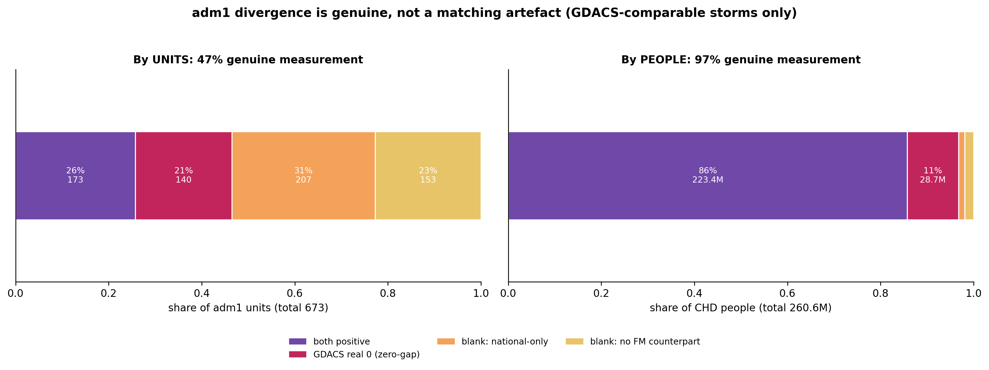
Figure 8.12: Why adm1 GDACS diverges from CHD, restricted to the GDACS-computed storms (the ~60 with a per-country footprint). Within them, most units and the large majority of people are genuine measurement divergence (both-positive + real zero-gap), not a matching artefact.

Going subnational, CHD-vs-GDACS drops from log-r 0.79 → 0.60 (median 0.43). Restricted to the GDACS-computed storms, most of the divergence is genuine measurement difference (both-positive + real zero-gap), not a matching artefact.

8.10 7. The full comparison — including true zeros

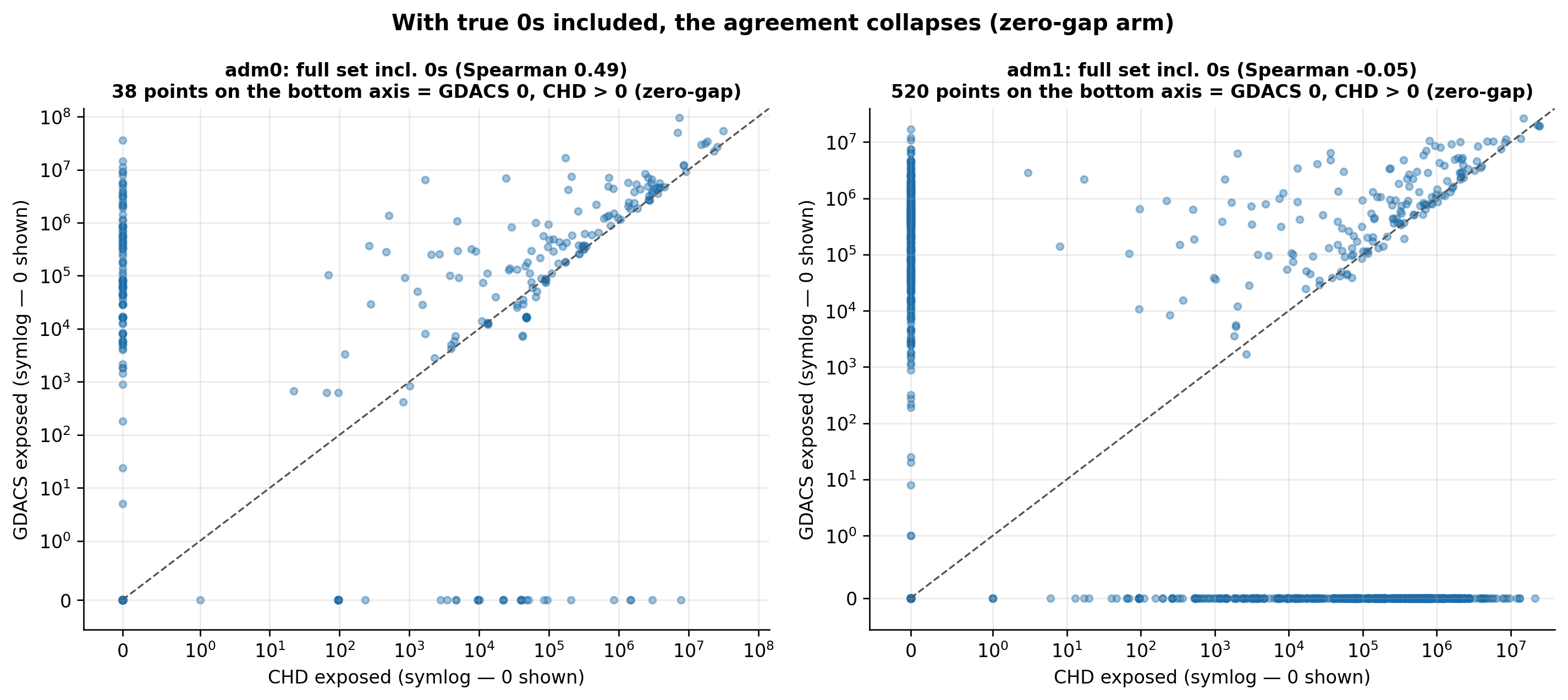
The magnitude view (§2–§3) drops zeros. With the five-case fills in place, the comparable set is simply every (storm, country, threshold) where GDACS is non-NaN — cases 1–3 (a positive value or a defensible 0), with the case-4/5 gaps excluded. Putting the true 0s back lets us ask a question the magnitude lens can’t: do the sources agree on who is exposed? First, the comparable set on symlog axes so the true 0s are visible:

from scipy.stats import spearmanr


def full_comparable(panel):
    # build_exposure already applied the five-case fills, so the comparable set
    # is just the cells where both sources are non-NaN (no manual fold-in).
    return overlap(panel, "chd", "gdacs")


fig, axes = plt.subplots(1, 2, figsize=(12, 5.4))
for ax, (panel, lvl) in zip(axes, ((panel0, "adm0"), (panel1, "adm1"))):
    d = full_comparable(panel)
    ax.scatter(d.chd_exposure, d.gdacs_exposure, s=14, alpha=0.4, color="#1b6ca8")
    lim = max(d.chd_exposure.max(), d.gdacs_exposure.max()) * 1.5
    ax.plot([0, lim], [0, lim], "--", color="#555", lw=1)
    ax.set_xscale("symlog", linthresh=1); ax.set_yscale("symlog", linthresh=1)
    ax.set_xlim(-0.5, lim); ax.set_ylim(-0.5, lim)
    ax.set_xlabel("CHD exposed (symlog — 0 shown)")
    ax.set_ylabel("GDACS exposed (symlog — 0 shown)")
    rho = spearmanr(d.chd_exposure, d.gdacs_exposure).statistic
    n_zg = int(((d.chd_exposure > 0) & (d.gdacs_exposure == 0)).sum())
    ax.set_title(f"{lvl}: full set incl. 0s (Spearman {rho:.2f})\n"
                 f"{n_zg} points on the bottom axis = GDACS 0, CHD > 0 (zero-gap)",
                 fontsize=10)
fig.suptitle("With true 0s included, the agreement collapses (zero-gap arm)",
             fontsize=12, fontweight="bold")
fig.tight_layout()
plt.show()

Figure 8.13: The full comparable set on symlog axes (true 0s shown — they sit on the axes). The both-positive cloud is off-axis; the arm along the bottom (GDACS true 0 while CHD > 0) is the defensible zero-gap. A rank correlation that includes the zeros stays low (panel titles), versus log-r 0.68 on positives only.

The question only the zeros can answer:

def kappa(pc, pg):
    po = (pc == pg).mean()
    pe = pc.mean() * pg.mean() + (1 - pc.mean()) * (1 - pg.mean())
    return (po - pe) / (1 - pe)


fig, axes = plt.subplots(1, 2, figsize=(12, 5))
for ax, (panel, lvl) in zip(axes, ((panel0, "adm0"), (panel1, "adm1"))):
    d = full_comparable(panel)
    pc = (d.chd_exposure > 0).astype(int)
    pg = (d.gdacs_exposure > 0).astype(int)
    cm = np.array([[((pc == 1) & (pg == 1)).sum(), ((pc == 1) & (pg == 0)).sum()],
                   [((pc == 0) & (pg == 1)).sum(), ((pc == 0) & (pg == 0)).sum()]])
    ax.imshow(cm, cmap="Blues")
    for i in range(2):
        for j in range(2):
            ax.text(j, i, f"{cm[i, j]:,}", ha="center", va="center", fontsize=13,
                    color="white" if cm[i, j] > cm.max() / 2 else "#222")
    ax.set_xticks([0, 1]); ax.set_xticklabels(["GDACS > 0", "GDACS = 0"])
    ax.set_yticks([0, 1]); ax.set_yticklabels(["CHD > 0", "CHD = 0"])
    ax.set_title(f"{lvl}: presence agreement "
                 f"{(pc == pg).mean()*100:.0f}% (κ={kappa(pc, pg):.2f})\n"
                 f"n={len(d):,} comparable units", fontsize=10.5)
fig.suptitle("Do the sources agree on WHO is exposed?  (full set, true 0s included)",
             fontsize=12, fontweight="bold")
fig.tight_layout()
plt.show()

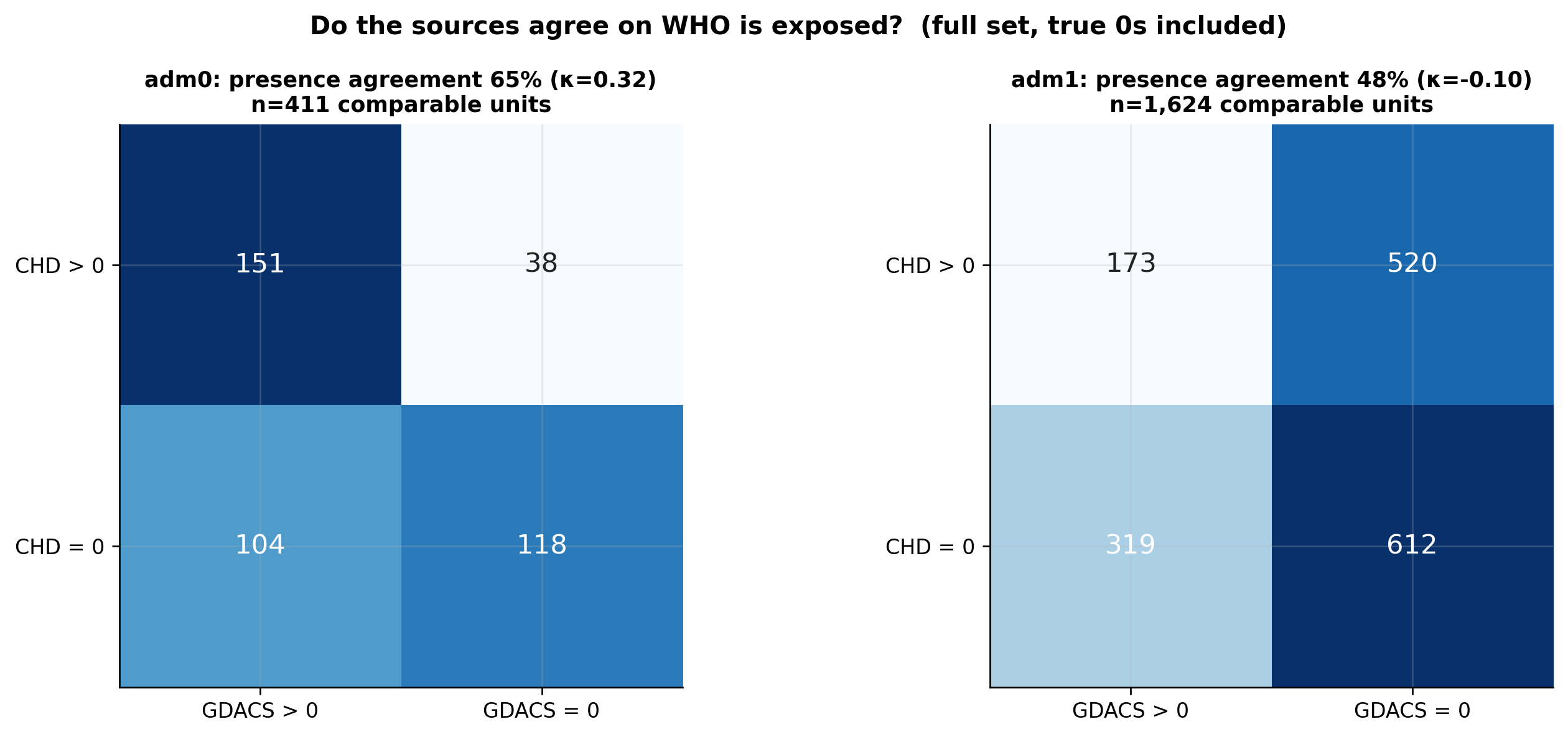
Figure 8.14: Do the sources agree on WHO is exposed? Confusion of CHD-exposed vs GDACS-exposed over the full comparable set (cases 1-3, true 0s included). Cohen’s κ is near zero — agreement on presence is barely better than chance. The off-diagonal (CHD>0, GDACS true 0) is a large cell.

With the true 0s in, the two sources agree on who is even exposed only about half the time (κ ≈ 0) — barely better than chance. The off-diagonal is dominated by the zero-gap: cells where CHD assigns exposure but GDACS computed a true 0. So the magnitude lens (§2–§3) and the presence lens tell the same story from two angles — CHD is the systematic low outlier on shared positives, and the two sources frequently disagree on whether a unit is exposed at all.

8.11 Caveats

• The pairwise correlations are not directly comparable — CHD-vs-GDACS, CHD-vs-ADAM and GDACS-vs-ADAM are computed on different, largely non-overlapping storm sets. ADAM’s small n (~44 storms) makes its statistics fragile.
• The per-country comparison is thin (~60 storms). GDACS’s getimpact per-country breakdown is -1 (“not computed”) for ~118 storms (its ~2016–2022 era). Those are NaN per country, not zeros — treating the -1s as 0 would manufacture a large fake zero-gap.
• GDACS still has a storm total for the missing storms. gettimeline computed a storm-wide total (Maria 11.6M, Matthew 18.3M) even where getimpact is -1; §5b recovers those at the storm-total grain, but a storm total cannot enter the per-country grid.
• adm1 magnitudes are matched-units-only, and the both-positive correlation describes a minority of the overlap — always report it alongside the zero-gap.
• Operational windows differ (GDACS 2015+, ADAM 2023+); coverage must be read on a same-era footing.

8.12 Headline

GDACS+ADAM are one source, and it produces a usable per-country exposure for only ~60 storms — the rest are data gaps (a storm total only) or genuine zeros. Where comparable, CHD reads about half of GDACS per shared unit (median ≈ 0.5), consistently at both the country and subnational level; and the two agree on who is exposed only about half the time (κ ≈ 0).

8.13 Appendix: comparing aggregate ratios across admin levels

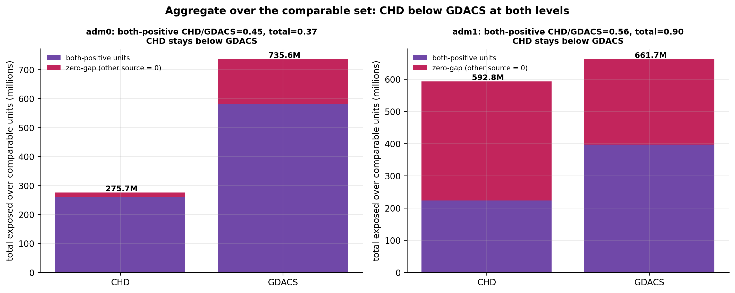
It is tempting to compare the aggregate CHD/GDACS ratio — total exposed summed over the comparable set — between adm0 and adm1. That comparison is not meaningful, because the comparable set is a different population of cells at each level. The aggregate runs over cells where both sources are non-NaN, and that overlap is selected differently at adm0 than at adm1. The robust magnitude figure is the both-positive ratio (≈ 0.5, §2–§3), not the aggregate.

fig, axes = plt.subplots(1, 2, figsize=(12, 4.8))
for ax, (panel, lvl) in zip(axes, ((panel0, "adm0"), (panel1, "adm1"))):
    d = full_comparable(panel)
    ce, ge = d.chd_exposure, d.gdacs_exposure
    bp = (ce > 0) & (ge > 0); zg = (ce > 0) & (ge == 0); gzg = (ce == 0) & (ge > 0)
    chd_bp, chd_zg = ce[bp].sum() / 1e6, ce[zg].sum() / 1e6
    gd_bp, gd_zg = ge[bp].sum() / 1e6, ge[gzg].sum() / 1e6
    ax.bar(0, chd_bp, color="#7048a8", label="both-positive units")
    ax.bar(0, chd_zg, bottom=chd_bp, color="#c2255c",
           label="zero-gap (other source = 0)")
    ax.bar(1, gd_bp, color="#7048a8")
    ax.bar(1, gd_zg, bottom=gd_bp, color="#c2255c")
    ax.text(0, chd_bp + chd_zg, f" {human(ce.sum())}", ha="center", va="bottom",
            fontsize=9, fontweight="bold")
    ax.text(1, gd_bp + gd_zg, f" {human(ge.sum())}", ha="center", va="bottom",
            fontsize=9, fontweight="bold")
    ax.set_xticks([0, 1]); ax.set_xticklabels(["CHD", "GDACS"])
    ax.set_ylabel("total exposed over comparable units (millions)")
    bp_ratio = ce[bp].sum() / ge[bp].sum(); tot_ratio = ce.sum() / ge.sum()
    ax.set_title(f"{lvl}: both-positive CHD/GDACS={bp_ratio:.2f}, "
                 f"total={tot_ratio:.2f}\nCHD stays below GDACS", fontsize=9.5)
    ax.legend(fontsize=8, frameon=False)
fig.suptitle("Aggregate over the comparable set: CHD below GDACS at both levels",
             fontsize=12, fontweight="bold")
fig.tight_layout()
plt.show()

Figure 8.15: Aggregate over the comparable set, split into both-positive units vs the zero-gap (where the other source is a true 0). CHD’s total stays below GDACS at both adm0 and adm1. The adm1 ratio is higher than adm0 only because the adm1 comparable set differs (decomposed below), not because of any real subnational coverage difference.

Decomposing the adm1 aggregate shows where its higher ratio comes from:

ov0 = overlap(panel0, "chd", "gdacs")
ov1 = overlap(panel1, "chd", "gdacs")
comp0 = set(zip(ov0.atcf_id, ov0.iso3, ov0.wind_speed_kt))
inc0 = [(s, i, k) in comp0 for s, i, k in
        zip(ov1.atcf_id, ov1.iso3, ov1.wind_speed_kt)]
ov1 = ov1.assign(inc0=inc0)
same = ov1[ov1.inc0]; extra = ov1[~ov1.inc0]
rows = [("adm0 — comparable countries", ov0.chd_exposure.sum(), ov0.gdacs_exposure.sum()),
        ("adm1 — same countries as adm0", same.chd_exposure.sum(), same.gdacs_exposure.sum()),
        ("adm1 — all comparable units", ov1.chd_exposure.sum(), ov1.gdacs_exposure.sum())]
tab = pd.DataFrame(rows, columns=["basis", "CHD_raw", "GDACS_raw"])
tab["CHD/GDACS"] = (tab.CHD_raw / tab.GDACS_raw).round(2)
tab["CHD"] = tab.CHD_raw.map(human); tab["GDACS"] = tab.GDACS_raw.map(human)
print(f"adm1 units in countries NOT in the adm0 comparable set: {len(extra)} units, "
      f"CHD {human(extra.chd_exposure.sum())}, GDACS {human(extra.gdacs_exposure.sum())}")
tab[["basis", "CHD", "GDACS", "CHD/GDACS"]].set_index("basis")

adm1 units in countries NOT in the adm0 comparable set: 731 units, CHD 327.8M, GDACS 0

Table 8.2

	CHD	GDACS	CHD/GDACS
basis
adm0 — comparable countries	275.7M	735.6M	0.37
adm1 — same countries as adm0	265.0M	661.7M	0.40
adm1 — all comparable units	592.8M	661.7M	0.90

Restricted to the same countries that are comparable at adm0, the ratio is essentially flat going to adm1 — CHD’s comparable total barely changes (it conserves across levels, adm0 ≈ Σ adm1). The higher all-comparable adm1 ratio comes entirely from subnational units in countries GDACS does not report at adm0: there GDACS is a 0 while CHD has people, so they enter the adm1 numerator with nothing in the denominator. That is a GDACS adm0-vs-adm1 reporting inconsistency (adm0 = NaN, adm1 = 0), not a subnational coverage signal — which is why magnitude should be read from the both-positive ratio, not the aggregate.