11  Appendix: ADAM, GDACS & CERF Allocation Overlap

This appendix documents the early work scoping ADAM (WFP) and GDACS as exposure sources for CERF Rapid Response allocation modelling. Both datasets were considered alongside the OCHA in-house exposure product; this chapter focuses on the question “can we use them to drive RR allocation modelling given CERF’s 2006 to 2023 temporal coverage?” Because of the limited overlap, the answer was no, and the main analysis uses the OCHA exposure dataset instead (see Data & Merge, which covers the storm ID matching that links CERF allocations to exposure).

A broader methodology-level comparison of OCHA vs GDACS, independent of CERF modelling constraints, is in OCHA vs GDACS: Exposure Method Comparison.

Code
import ocha_stratus as stratus
import pandas as pd
import matplotlib.pyplot as plt
import matplotlib.ticker as mticker
import numpy as np
from dotenv import load_dotenv

load_dotenv()

df_cerf = stratus.load_csv_from_blob(
    "ds-storm-impact-harmonisation/processed/cerf-storms-with-sids-2024-02-27.csv"
)
df_adam = stratus.load_csv_from_blob(
    "ds-cyclone-exposure/adam_historical_national_exposure.csv"
)
df_gdacs = stratus.load_csv_from_blob(
    "ds-cyclone-exposure/gdacs_historical_national_exposure.csv"
)

11.1 ADAM (WFP)

ADAM provides population exposure at three wind speed thresholds: 60, 90, and 120 km/h.

Code
print(f"Rows: {len(df_adam)} | Storms: {df_adam['sid'].nunique()}")
print(f"Seasons: {int(df_adam['season'].min())}{int(df_adam['season'].max())}")
print(f"Date range: {df_adam['from_date'].min()}{df_adam['from_date'].max()}")
print(f"Countries: {df_adam['iso3'].nunique()}")
Rows: 194 | Storms: 47
Seasons: 2023–2025
Date range: 2023-08-16T15:00:00 → 2025-10-21T15:00:00
Countries: 38

11.2 GDACS

GDACS provides population exposure at two wind speed thresholds: 34 kt and 64 kt.

Code
print(f"Rows: {len(df_gdacs)} | Storms: {df_gdacs['sid'].nunique()}")
print(f"Seasons: {int(df_gdacs['season'].min())}{int(df_gdacs['season'].max())}")
print(f"Date range: {df_gdacs['from_date'].min()}{df_gdacs['from_date'].max()}")
print(f"Countries: {df_gdacs['iso3'].nunique()}")
Rows: 574 | Storms: 177
Seasons: 2015–2025
Date range: 2015-07-11T15:00:00 → 2025-10-21T15:00:00
Countries: 56

11.3 GDACS Data Completeness Issue

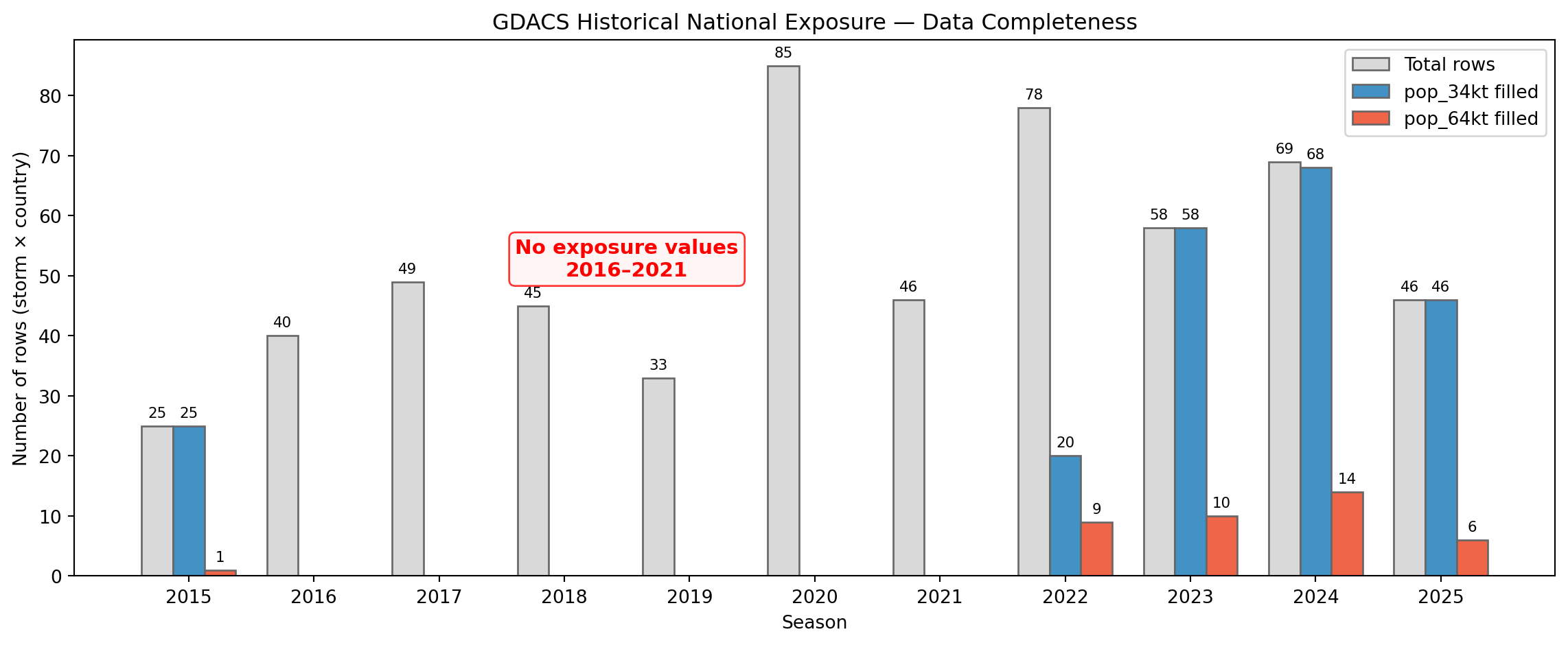
GDACS has rows going back to 2015, but the actual population exposure values are missing for 2016–2021. This is likely a pipeline issue — the storm metadata was ingested but exposure calculations were not run for those years.

Code
seasons = sorted(df_gdacs["season"].unique())
stats = []
for s in seasons:
    sub = df_gdacs[df_gdacs["season"] == s]
    stats.append({
        "season": int(s),
        "total": len(sub),
        "pop_34kt_filled": sub["pop_34kt"].notna().sum(),
        "pop_64kt_filled": sub["pop_64kt"].notna().sum(),
    })
stats_df = pd.DataFrame(stats)

x = np.arange(len(stats_df))
width = 0.25

fig, ax = plt.subplots(figsize=(12, 5))
bars1 = ax.bar(x - width, stats_df["total"], width, label="Total rows", color="#d9d9d9", edgecolor="#666")
bars2 = ax.bar(x, stats_df["pop_34kt_filled"], width, label="pop_34kt filled", color="#4292c6", edgecolor="#666")
bars3 = ax.bar(x + width, stats_df["pop_64kt_filled"], width, label="pop_64kt filled", color="#ef6548", edgecolor="#666")

for bars in [bars1, bars2, bars3]:
    for bar in bars:
        h = bar.get_height()
        if h > 0:
            ax.text(bar.get_x() + bar.get_width() / 2, h + 1, str(int(h)),
                    ha="center", va="bottom", fontsize=8)

ax.set_xlabel("Season")
ax.set_ylabel("Number of rows (storm × country)")
ax.set_title("GDACS Historical National Exposure — Data Completeness")
ax.set_xticks(x)
ax.set_xticklabels(stats_df["season"].astype(str))
ax.legend()
ax.annotate(
    "No exposure values\n2016–2021", xy=(3.5, 50),
    fontsize=11, ha="center", color="red", fontweight="bold",
    bbox=dict(boxstyle="round,pad=0.3", facecolor="#fff3f3", edgecolor="red", alpha=0.8),
)
plt.tight_layout()
plt.show()

GDACS exposure data completeness by season. Rows exist for 2016–2021 but contain no exposure values.

The pop_64kt column is also sparse even in years with data — only filled for the most intense storms where winds exceeded 64 kt in populated areas.

Code
stats_df["pop_34kt_pct"] = (stats_df["pop_34kt_filled"] / stats_df["total"] * 100).round(0).astype(int).astype(str) + "%"
stats_df["pop_64kt_pct"] = (stats_df["pop_64kt_filled"] / stats_df["total"] * 100).round(0).astype(int).astype(str) + "%"
stats_df[["season", "total", "pop_34kt_filled", "pop_34kt_pct", "pop_64kt_filled", "pop_64kt_pct"]]
season total pop_34kt_filled pop_34kt_pct pop_64kt_filled pop_64kt_pct
0 2015 25 25 100% 1 4%
1 2016 40 0 0% 0 0%
2 2017 49 0 0% 0 0%
3 2018 45 0 0% 0 0%
4 2019 33 0 0% 0 0%
5 2020 85 0 0% 0 0%
6 2021 46 0 0% 0 0%
7 2022 78 20 26% 9 12%
8 2023 58 58 100% 10 17%
9 2024 69 68 99% 14 20%
10 2025 46 46 100% 6 13%

11.4 Exposure Column Semantics

A critical finding: ADAM and GDACS use different conventions for their exposure columns.

11.4.1 ADAM: Binned (not cumulative)

The ADAM columns represent population within a wind speed band, not everyone above a threshold:

  • pop_60kmh → population exposed to 60–90 km/h only
  • pop_90kmh → population exposed to 90–120 km/h only
  • pop_120kmh → population exposed to ≥ 120 km/h

Evidence: pop_60kmh < pop_90kmh in many rows, which is impossible if cumulative.

Code
adam_check = df_adam[["sid", "iso3", "pop_60kmh", "pop_90kmh", "pop_120kmh"]].dropna()
n_violation = (adam_check["pop_60kmh"] < adam_check["pop_90kmh"]).sum()
print(f"Rows where pop_60kmh < pop_90kmh: {n_violation} of {len(adam_check)}")
print("(Impossible if cumulative — confirms these are bins)\n")
adam_check[adam_check["pop_60kmh"] < adam_check["pop_90kmh"]].head(5)
Rows where pop_60kmh < pop_90kmh: 17 of 97
(Impossible if cumulative — confirms these are bins)
sid iso3 pop_60kmh pop_90kmh pop_120kmh
0 2025294N14290 BHS 9764 11808.0 4166.0
4 2025294N14290 CUB 1070326 1953526.0 1834084.0
63 2024309N13283 CUB 1288088 2733790.0 597297.0
92 2024225N14313 VGB 0 26087.0 0.0
115 2024181N09320 CYM 1791 56112.0 0.0

To convert to cumulative (≥ threshold):

Code
df_adam["pop_gte_60kmh"] = df_adam["pop_60kmh"].fillna(0) + df_adam["pop_90kmh"].fillna(0) + df_adam["pop_120kmh"].fillna(0)
df_adam["pop_gte_90kmh"] = df_adam["pop_90kmh"].fillna(0) + df_adam["pop_120kmh"].fillna(0)
df_adam["pop_gte_120kmh"] = df_adam["pop_120kmh"].fillna(0)

# Verify monotonicity after conversion
assert (df_adam["pop_gte_60kmh"] >= df_adam["pop_gte_90kmh"]).all()
assert (df_adam["pop_gte_90kmh"] >= df_adam["pop_gte_120kmh"]).all()
print("Cumulative conversion verified: pop_gte_60 >= pop_gte_90 >= pop_gte_120")
Cumulative conversion verified: pop_gte_60 >= pop_gte_90 >= pop_gte_120

11.4.2 GDACS: Cumulative

GDACS columns are already cumulative (≥ threshold):

  • pop_34kt → all population exposed to ≥ 34 kt
  • pop_64kt → all population exposed to ≥ 64 kt
Code
gdacs_check = df_gdacs[["pop_34kt", "pop_64kt"]].dropna()
assert (gdacs_check["pop_34kt"] >= gdacs_check["pop_64kt"]).all()
print(f"Confirmed: pop_34kt >= pop_64kt in all {len(gdacs_check)} non-null rows")
Confirmed: pop_34kt >= pop_64kt in all 37 non-null rows

11.4.3 Cross-Validation

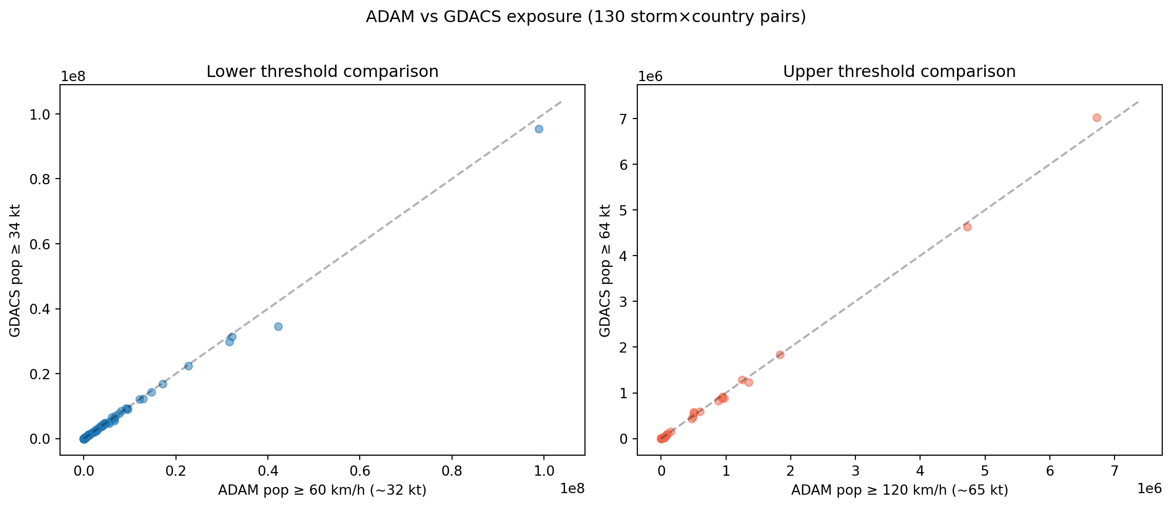
Since 60 km/h ≈ 32 kt and 120 km/h ≈ 65 kt, we can compare the two sources for storms that appear in both datasets.

Code
common = df_adam[["sid", "iso3", "pop_gte_60kmh", "pop_gte_120kmh"]].merge(
    df_gdacs[["sid", "iso3", "pop_34kt", "pop_64kt"]],
    on=["sid", "iso3"],
)
common = common.dropna(subset=["pop_gte_60kmh", "pop_34kt"])
# Remove sentinel -1 values
common = common[(common["pop_34kt"] >= 0) & (common["pop_gte_60kmh"] >= 0)]

fig, (ax1, ax2) = plt.subplots(1, 2, figsize=(12, 5))

ax1.scatter(common["pop_gte_60kmh"], common["pop_34kt"], alpha=0.5, s=30)
lim = max(common["pop_gte_60kmh"].max(), common["pop_34kt"].max()) * 1.05
ax1.plot([0, lim], [0, lim], "k--", alpha=0.3)
ax1.set_xlabel("ADAM pop ≥ 60 km/h (~32 kt)")
ax1.set_ylabel("GDACS pop ≥ 34 kt")
ax1.set_title("Lower threshold comparison")
ax1.ticklabel_format(style="scientific", scilimits=(0, 0))

common_64 = common.dropna(subset=["pop_gte_120kmh", "pop_64kt"])
common_64 = common_64[(common_64["pop_64kt"] >= 0) & (common_64["pop_gte_120kmh"] >= 0)]
ax2.scatter(common_64["pop_gte_120kmh"], common_64["pop_64kt"], alpha=0.5, s=30, color="#ef6548")
if len(common_64) > 0:
    lim2 = max(common_64["pop_gte_120kmh"].max(), common_64["pop_64kt"].max()) * 1.05
    ax2.plot([0, lim2], [0, lim2], "k--", alpha=0.3)
ax2.set_xlabel("ADAM pop ≥ 120 km/h (~65 kt)")
ax2.set_ylabel("GDACS pop ≥ 64 kt")
ax2.set_title("Upper threshold comparison")
ax2.ticklabel_format(style="scientific", scilimits=(0, 0))

plt.suptitle(f"ADAM vs GDACS exposure ({len(common)} storm×country pairs)", y=1.02)
plt.tight_layout()
plt.show()

Cross-validation of ADAM vs GDACS exposure estimates for overlapping storms. Dashed line is y=x.

11.5 Temporal Coverage & CERF Overlap

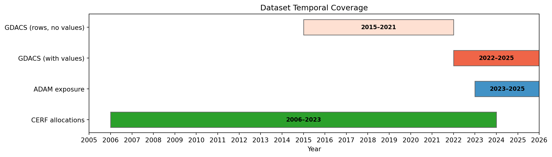
The fundamental challenge: CERF allocations and exposure estimates barely overlap in time.

Code
fig, ax = plt.subplots(figsize=(12, 3.5))

datasets = [
    ("CERF allocations", 2006, 2023, "#2ca02c"),
    ("ADAM exposure", 2023, 2025, "#4292c6"),
    ("GDACS (with values)", 2022, 2025, "#ef6548"),
    ("GDACS (rows, no values)", 2015, 2021, "#fee0d2"),
]

for i, (name, start, end, color) in enumerate(datasets):
    ax.barh(i, end - start + 1, left=start, height=0.5, color=color, edgecolor="#666", label=name)
    ax.text(start + (end - start + 1) / 2, i, f"{start}{end}", ha="center", va="center", fontsize=9, fontweight="bold")

ax.set_yticks(range(len(datasets)))
ax.set_yticklabels([d[0] for d in datasets])
ax.set_xlabel("Year")
ax.set_title("Dataset Temporal Coverage")
ax.set_xlim(2005, 2026)
ax.xaxis.set_major_locator(mticker.MultipleLocator(1))
plt.tight_layout()
plt.show()

Temporal coverage of each dataset. The CERF allocation period (2006–2023) has almost no overlap with years where exposure data exists.

11.6 Join Results

Joining CERF (with valid sids) to the combined exposure data on sid + iso3:

Code
iso2_to_iso3 = {
    "AG": "ATG", "BD": "BGD", "BO": "BOL", "BS": "BHS", "CO": "COL",
    "CU": "CUB", "DJ": "DJI", "DM": "DMA", "DO": "DOM", "FJ": "FJI",
    "GH": "GHA", "GT": "GTM", "HN": "HND", "HT": "HTI", "KM": "COM",
    "KP": "PRK", "LA": "LAO", "MG": "MDG", "ML": "MLI", "MM": "MMR",
    "MW": "MWI", "MZ": "MOZ", "NI": "NIC", "PH": "PHL", "PK": "PAK",
    "RW": "RWA", "SD": "SDN", "SV": "SLV", "UG": "UGA", "VN": "VNM",
    "VU": "VUT", "ZW": "ZWE",
}
df_cerf["iso3"] = df_cerf["iso2"].map(iso2_to_iso3)

# Build combined exposure
df_gdacs_r = df_gdacs.rename(columns={"pop_34kt": "pop_gte_34kt", "pop_64kt": "pop_gte_64kt"})
exposure = df_gdacs_r[["sid", "iso3", "pop_gte_34kt", "pop_gte_64kt"]].merge(
    df_adam[["sid", "iso3", "pop_gte_60kmh", "pop_gte_90kmh", "pop_gte_120kmh"]],
    on=["sid", "iso3"],
    how="outer",
)

cerf_valid = df_cerf.dropna(subset=["sid"])
merged = cerf_valid.merge(exposure, on=["sid", "iso3"], how="left")

exposure_cols = ["pop_gte_34kt", "pop_gte_64kt", "pop_gte_60kmh", "pop_gte_90kmh", "pop_gte_120kmh"]
has_any = merged.dropna(subset=exposure_cols, how="all")

print(f"CERF rows total:          {len(df_cerf)}")
print(f"CERF rows with sid:       {len(cerf_valid)}")
print(f"  → matched with exposure: {len(has_any)}")
print(f"  → no exposure data:      {len(merged) - len(has_any)}")
print(f"\nUnique storms with sid: {cerf_valid['sid'].nunique()}")
print(f"  → with exposure:  {has_any['sid'].nunique()}")
CERF rows total:          82
CERF rows with sid:       58
  → matched with exposure: 1
  → no exposure data:      57

Unique storms with sid: 44
  → with exposure:  1
Code
if len(has_any) > 0:
    print("Matched rows:")
    display(has_any[["Country", "iso3", "sid", "allocation_year", "Amount in US$"] + exposure_cols])
Matched rows:
Country iso3 sid allocation_year Amount in US$ pop_gte_34kt pop_gte_64kt pop_gte_60kmh pop_gte_90kmh pop_gte_120kmh
6 Cuba CUB 2022266N12294 2022 7827734 NaN 655778.0 NaN NaN NaN

11.7 Summary

Metric Value
CERF allocations 82 rows (2006–2023)
CERF with storm ID 58 of 82 rows (71%)
ADAM exposure range 2023–2025 (47 storms)
GDACS exposure range 2015–2025 rows, 2022–2025 usable (60 storms with values)
CERF × Exposure matches ~1 row

Key blockers:

  1. GDACS 2016–2021 gap — rows exist but exposure values are null (pipeline issue?)
  2. ADAM only starts 2023 — no overlap with bulk of CERF data (2006–2022)
  3. CERF missing sids — 29% of allocations can’t be joined at all

Filling the GDACS 2016–2021 exposure gap would immediately unlock 6 more storms (11 CERF allocation rows). Extending exposure estimates further back to 2006 would maximise the usable dataset.